
Decoding (ASR Part 4)
19 Dec 2018Link to the start of ASR series: Automatic Speech Recognition (ASR Part 0)
Now that we have explored Acoustic Modeling and Language Modeling, the next logical question is, how do we put these things together? Running both AM and LM and combining the results into a list of hypothesis is called as the Decoding Process and this is harder than it looks mainly because of latency and speed concerns which have an adverse effect on RTF.
Decoding Speed
Decoding speed is usually measured with respect to a real-time factor (RTF). A RTF of 1.0 means that the system processes the data in real-time, takes ten seconds to process ten seconds of audio. Factors above 1.0 indicate that the system needs more time to process the data (Used in meeting transcriptions). When the RTF is below 1.0, the system processes the data more quickly than it arrives. For instance, when performing a remote voice query on the phone, network congestion can cause gaps and delays in receiving the audio at the server. If the ASR system can process data in faster than real-time, it can catch up after the data arrives, hiding the latency behind the speed of the recognition system.
The solution to a majority of latency issues in computer engineering lies in data structures. ASR decoding is no different. In order to make decoding easier, we represent both the AM and the LM as Weighted Finite State Transducers (WFSTs). This brings with it all the capabilities of WFST operations to AM and LM in order to combine them.
Before we dive into WFST, there are other data structures that we need to be introduced to.
Finite State Acceptor (FSA)
Finite representation of a possibly infinite set of strings. It is a Finite State Machine (FSM) where there are states (INITIAL and FINAL). Transition from one state to the other is by consuming a letter (let us call this input).
Weighted Finite State Acceptor (WFSA)
WFSA is similar to FSA except that there is a cost associated with each state change. Cost is multiplied along one path and added across paths. Therefore, even though there are multiple ways of going from the initial state to the final state, we take the path with min cost.
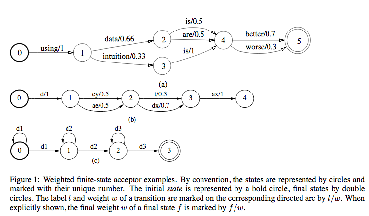
In the above figure, we can see 3 types of applications of WFSAs in ASRs.
- Figure 1(a): Finite state language model
- Figure 1(b): Possible pronunciations of the word \(\text{data}\) used in the language model
- Figure 1(c): 3-distribution-HMM structure for one phone, with the labels along a complete path specifying legal strings of acoustic distributions for that phone.
Finite State Transducer (FST)
FST is similar to FSA except that for each arc, we have both input and output symbols. For the corresponding state transition, we consume the input symbol and emit the output symbol.
Weighted Finite State Transducer (WFST)
WFST is similar to FST except that there is a cost associated with each state change. All the operations on cost that we perform on WFSA are applicable here too.
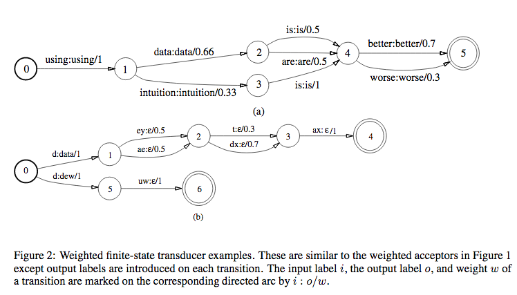
The figure above is same as the WFSA but with input:output on each state instead of just input. \(\epsilon\) is a null symbol.
Now that we know what FSA, WFSA, FST and WFST are, why do we choose WFST over other data structures to represent models in our ASR? WFST (which is a transducer) can represent a relationship between two levels of representation, for eg, between phones and words (like figure 2(b)) or between HMMs and context-independent phones.
- WFST Union: Combine transducers in parallel
- WFST Concatenation: Combine transducers in series
- Kleene Closure: Combine transducers with arbitrary repetition (With * or +)
Operations on WFSTs
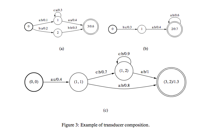
- Composition
If there are two transducers \(T_{1}\) and \(T_{2}\) and their composition is \(T\), we represent \(T=T_{1} \circ T_{2}\). If \(T_{1}\) takes \(u\) as input and gives \(v\) as output and \(T_{2}\) takes \(v\) as input and gives \(w\) was output, then \(T\) takes \(u\) as input and gives \(w\) as output. Weights in \(T\) is computed from the weights in \(T_{1}\) and \(T_{2}\) (maybe product (in case of prob) or sum (in case of log)).
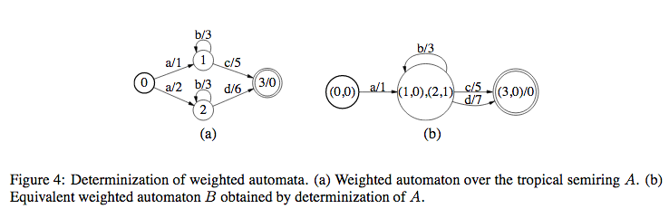
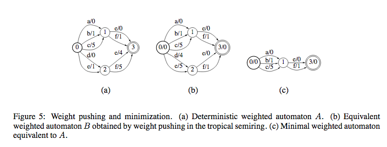
- Determinization
In this, WFSTs should satisfy the following conditions:
- From any state, for a given input, there should be only one transition
- No \(\epsilon\) symbols in input
The above conditions make it easier to compute determinization since from each state, we have only one transition for one input symbol.
- Minimization
This is to simplify the structure of the WFST.
WFST in Speech
WFSTs are used in the Decoding Stage. (WFST Speech Decoders). WFST is a way of representing HMMs, statistical language models, lexicons etc.
There are four principal models for speech recognition:
-
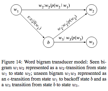
Word Level Grammar\((G)\): In \(G\), every word is considered to be a state. If we take a bigram model, there is a transition from \(w_{1}\) to \(w_{2}\) for every bigram \(w_{1}w_{2}\) in the corpus. The weight for this transition will be \(-log(p(w_{2}|w_{1}))\). We use \(\epsilon\) to represent unseen bigrams, for eg, \(w_{1}w_{3}\)
- Pronunciation Lexicon\((L)\): This transducer is non determinizable due to the following reasons:
- Homophones: Different words are pronounced the same, and hence will have the same sequence of phones.
- First word of the output string might not be known before the entire phone string is scanned: For eg, if we take the sequence of phones (corresponding to the word \(\text{"carla"}\)), we cannot say that the word is \(\text{"car"}\) before consuming the entire sequence.
In order to overcome this, we use a special symbol
#_{0}to mark the end of phonetic transcription of a word. In order to distinguish between homophones, we use other symbols such as#_{1}...#_{k-1}. For eg, \(\text{"red"}\) isr eh d #_{0}and \(\text{"read"}\) isr eh d #_{1}. - Context Dependency Transducer\((C)\): We denote context dependent units as
phone/leftcontext_rightcontext. - HMM Transducer\((H)\)
Consider the WFSTs in Figure 2. Figure 2(a) is the grammar \(G\) and in Figure 2(b) we have pronunciation lexicons \(L\). If we do a composition of these two transducers, we get a new transducer that takes phones as input and gives words as output (These words are restricted to the grammar \(G\) since \(G\) can’t accept any other words). So, we get \(L \circ G\).
The above composition is just a context independent substitution (Monophone model).
In order to get context dependent substitution, we again use composition on top of context independent substitution (called Triphone model).
Let us take the word \(\text{"cat"}\) as an example. The sequence of phonemes for this word is \(k\), \(\text{ae}\), \(t\). Let us assume that the notation \(\text{ae/k_t}\) represents a triphone model for \(\text{ae}\) with left context \(k\) and right context \(t\).
We have the following state transitions for the triphone model.
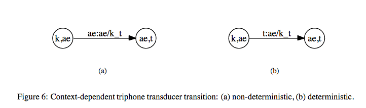
The above transducer that maps context independent phones to context dependent phones is denoted by \(C\). Hence, we get \(C \circ (L \circ G)\).
After this, we perform Determinization and Minimization on this.
\[N = min(det(C \circ (L \circ G)))\]Adding HMM to model the input distribution, WFST for speech recognition can be represented as a transducer which maps from distributions to words strings restricted to G.
\[H \circ (C \circ (L \circ G))\]