Interpreting Machine Learning Models - Part 5

16 Sep 2019

Link to start of the blog series: Interpretable ML

Type 2 : Model Agnostic Interpretation (Continued)

	Interpretablility	Accuracy
Complex Models	No	Yes
Simple Models	Yes	No

1. Shapely Values

   Lloyd Shapely, a Nobel Prize winner in 2012, came up with a cooperative game theory to distribute profits fairly. Basic premise is that if a group of people come together to play a cooperative game and win some money, how do we distribute this winnings fairly among the players? The individual players themselves interact differently to achieve the outcome and therefore how do we decide the contribution of each member to the collective objective fairly?

   A prediction can be explained by assuming that each feature value of the instance is a “player” in a game where the prediction is the payout. Shapley values – a method from coalitional game theory – tells us how to fairly distribute the “payout” among the features.

   Let us take the following example: We have a trained machine learning model to predict apartment prices. For a certain apartment it predicts €300,000 and you need to explain this prediction. The apartment has a size of 50 m^2, is located on the 2nd floor, has a park nearby and cats are banned. The average prediction for all apartments is €310,000. How much has each feature value contributed to the prediction compared to the average prediction?

   The feature values park-nearby, cat-banned, area-50 and floor-2nd worked together to achieve the prediction of €300,000. Our goal is to explain the difference between the actual prediction (€300,000) and the average prediction (€310,000): a difference of -€10,000.

   How do we calculate the Shapley value for one feature? The Shapley value is the average marginal contribution of a feature value across all possible coalitions. The following list shows all coalitions of feature values that are needed to determine the Shapley value for cat-banned. The first row shows the coalition without any feature values. The other rows show different coalitions with increasing coalition size, separated by “+”. All in all, the following coalitions are possible:

   • No feature values
   • park-nearby
   • size-50
   • floor-2nd
   • park-nearby + size-50
   • park-nearby + floor-2nd
   • size-50 + floor-2nd
   • park-nearby + size-50 + floor-2nd

   For each of these coalitions we compute the predicted apartment price with and without the feature value cat-banned and take the difference to get the marginal contribution. The Shapley value is the (weighted) average of marginal contributions. We replace the feature values of features that are not in a coalition with random feature values from the apartment dataset to get a prediction from the machine learning model.

   Accurate calculation of Shapely Values is a NP-Hard problem. Hence, we come up with a way of estimating it and one of the ways is SHAP.

2. SHAP (SHapley Additive exPlanations)

   

   

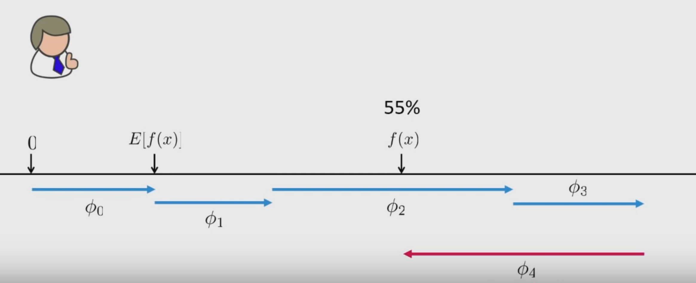
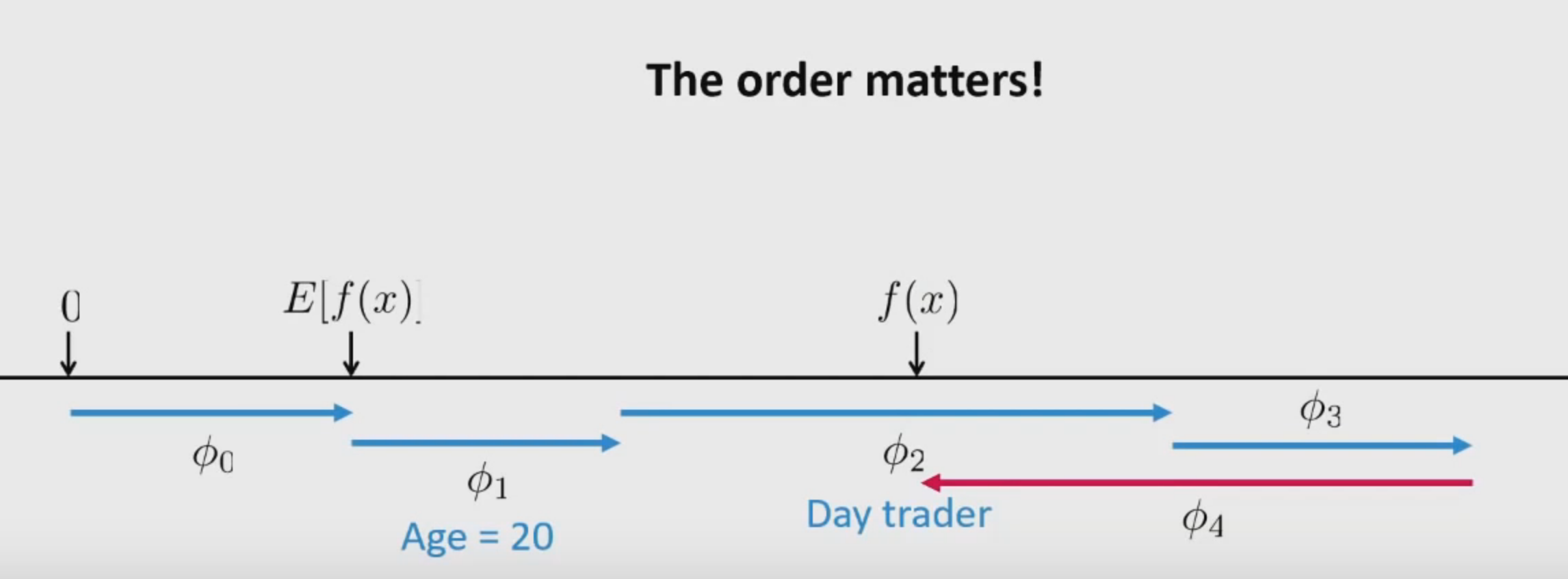
   Here, \(\phi\) is the feature attribution function that estimates feature importance.

   • Base Rate: Expectation of the model i.e mean of all predictions over the training data. \(E\left [ f(x) \right ]\)
   • Change in rate given a feature \(x_{1}\):
   \[E\left [ f(x) \right | x_{1}]\]
   • Change in rate given features \(x_{1}, x_{2}, x_{3}\):
   \[E\left [ f(x) \right | x_{1}, x_{2}, x_{3}]\]

   The main assumption is that: \(x_{1}\), \(x_{2}\) and \(x_{3}\) are conditionally independent.

   • Using LIME principles to estimate Shapely Values:
     • LIME uses a local kernel with a loss minimization function (an exponentially smoothed kernel) with regularization. We have to pick a loss function, regularizer and a local kernel. If you remember, from the previous post on LIME, I stated that this is a point of weakness of LIME as they were chosen heuristically.
     • LIME trains a linear model with the heuristic parameters. SHAP proposes that instead of using these heuristics, we can use Shapely Values (estimated through linear models) with a theoretical basis which obey the Shapely Principles.

   

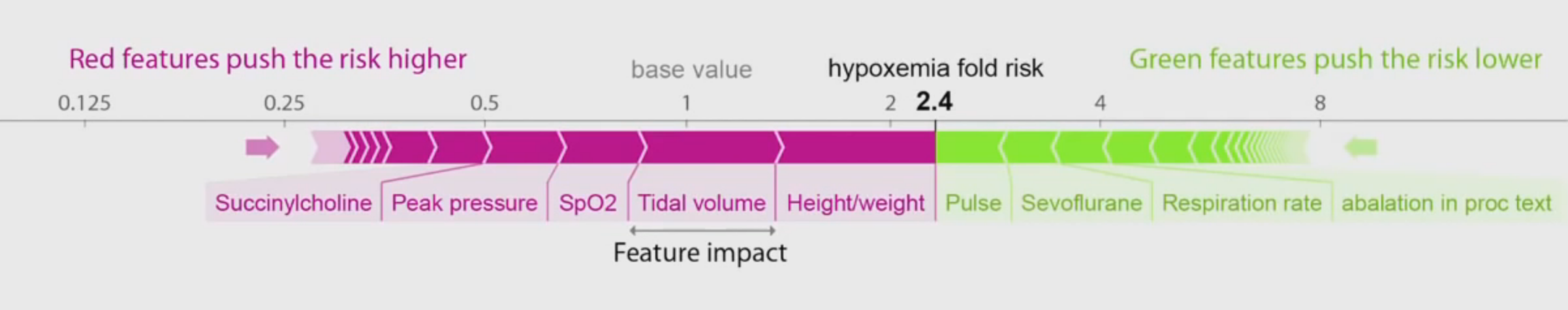
   An important thing to note here is that SHAP is not causal. It has scope for future work here. But, explainability is not causality i.e we are just explaining why a model gave a particular result without asserting that these features cause these outputs. A very important distinction.

   • More information about SHAP can be found at this talk by Lundberg, the creator of SHAP.
   • Link to the paper: A Unified Approach to Interpreting Model Predictions
   • Github Source

Interpreting Machine Learning Models - Part 4

15 Sep 2019

Link to start of the blog series: Interpretable ML

Type 2 : Model Agnostic Interpretation (Continued)

1. Feature Importance

   We measure the relative importance of a feature by permuting it’s values and observing it’s effect on the prediction. If the feature is “important” to the prediction, then the prediction changes drastically when the feature value is changed. Conversely, if the feature is relatively “unimportant”, then permuting the value of the feature will have negligible effect on the predicted value.

   NOTE: We still assume that the features are not correlated.

2. Global Surrogate

   Here, we solve a machine learning problem with more machine learning! If the black-box model is too complex to be interpreted, then we train a simple, interpretable model to mimick the bigger, complex model.

   This is an area of active research in machine learning, engendered not just by a need for interpretability, but also by a need to reduce model sizes. As the models get more and more complex, they grow in size too and contain millions of parameters. This makes it harder to deploy these models on memory-constrained devices such as phones and IoT devices. Therefore, we develop small ML models which can probe the complex model infinitely. Therefore, the smaller model trains to mimick the bigger model by observing how the prediction changes when the input is changed. These research endeavours have been surprisingly successful. The same approach is used in this case, where we train a smaller, interpretable model to mimick the bigger model and hence, we can interpret the outputs.

   This smaller model is called as a “surrogate” of the bigger model and more accurately, it is called as “global surrogate” as it mimicks the entire feature space of the bigger model. This is in contrast to “local surrogates” which is explored in the next section, where the surrogate is trained only on a local sub space of the bigger model and is used to interpret a single prediction.

3. Local Surrogate (LIME)

   Local interpretable model-agnostic explanations (LIME) focuses on training local surrogate models to interpret individual predictions instead of the entire model. This follows a similar principle of Feature Importance, where we generate a new dataset by perturbing the given input. The exact steps are outlined below:

   • Select the instance for which you want to have an explanation of its black box prediction.
   • Perturb your dataset and get the black box predictions for these new points. Similar to permuting only a single feature in Feature Importance, here we perturb the given vector by changing all the features.
   • Weight the new samples according to their proximity to the instance of interest. This is to give higher importance to generated instances which are closer to the instance of interest. This can be done by any similarity or distance metric. LIME uses an exponential smoothing kernel. A smoothing kernel is a function that takes two data instances and returns a proximity measure. The kernel width determines how large the neighborhood is: A small kernel width means that an instance must be very close to influence the local model, a larger kernel width means that instances that are farther away also influence the model.
   • Train a weighted, interpretable model on the dataset with the variations.
   • Explain the prediction by interpreting the local model.

   How do you get the variations of the data? This depends on the type of data, which can be either text, image or tabular data. For text and images, the solution is to turn single words or super-pixels on or off. In the case of tabular data, LIME creates new samples by perturbing each feature individually, drawing from a normal distribution with mean and standard deviation taken from the feature.

   • LIME for Tabular Data:
     • Tabular data is when the training data is in the form a table where each row is a training instance and each column is a feature.
     • The problem here, is how do we generate data close to the instance that we are interested in? Even though LIME uses exponential smoothing function with a kernel width of 0.75 times the square root of the number of columns of the training data, there is no explanation why.
   • LIME for Text:
     • Variations of the data are generated differently: Starting from the original text, new texts are created by randomly removing words from the original text. The dataset is represented with binary features for each word. A feature is 1 if the corresponding word is included and 0 if it has been removed.
   • LIME for Images:
     • LIME for images works differently than LIME for tabular data and text. Intuitively, it would not make much sense to perturb individual pixels, since many more than one pixel contribute to one class. Randomly changing individual pixels would probably not change the predictions by much. Therefore, variations of the images are created by segmenting the image into “superpixels” and turning superpixels off or on. Superpixels are interconnected pixels with similar colors and can be turned off by replacing each pixel with a user-defined color such as gray. The user can also specify a probability for turning off a superpixel in each permutation.

Interpreting Machine Learning Models - Part 3

31 Jul 2019

Link to start of the blog series: Interpretable ML

Type 2 : Model Agnostic Interpretation

In the previous blog post, we explored various inherently interpretable machine learning models. In this blog post, we will explore various methods of interpretation without any dependency on the type of ML model.

Given an opportunity, we can stick with only inherently ML models. Unfortunately, we have access to innumerable other ML models which are much better than the inherently interpretable ML models. We cannot abandon the former in favor of the latter. Also, having methods to induce interpretability of ML models without relying on the type of model allows us, as developers, to experiment with any number of variations of models without sacrificing interpretability.

1. Partial Dependency Plot (PDP)

   In layman terms, this plot illustrates the correlation between a feature and target. It illustrates how the target variable changes with change in feature variable value.

   This requires us to know something called as marginalisation. Assume we have 4 variables \(x,y,z\) and we have a function \(f\). This function \(f\) can be represented as

   \(f(x,y) = \int f(x,y,z) dz\).

   If \(z\) was a discrete variable, then integration is replaced by the summation symbol. By integrating (or summing) over all values of \(z\), we have marginalised the function \(f\) over \(z\) and now we get a relation between \(x\), \(y\) and \(f\) (i.e \(f(x,y)\)) only without any dependency on \(z\).

   This concept is utilised in PDP, where \(\text{set S}\) is the set of all features that we are interested in and \(\text{set C}\) is the set of all features that we are not interested in.

   \(S \cup C = \text{All Features}\).

   By marginalising over the features in \(\text{set C}\), we get the relation between \(\text{set S}\) and the ML model.

   To illustrate, let us assume that the features are \(a\), \(b\), \(c\), \(d\) and the ML model is \(f\).

   The output of the ML model is given by,

   \[y = f(a,b,c,d)\]

   Now, we would like to plot a PDP between \(a\) and the ML model (i.e) we would like to know the how \(a\) affects the model output.

   Therefore, marginalising over all the other features,

   \[f(a) = \int f(a,b,c,d) db dc dd\]

   Now, we have the relation between \(f(a)\) and \(f(a,b,c,d)\). This is nothing but the PDP plot.

   This works for all numerical features. When it comes to categorical features, it becomes simpler because we just need to expand on all the combinations of the categorical features. For example, is an ML model relies on “temperature” and “weather” to predict water sales, we can just set the “weather” variable to “summer”, “spring”, “autumn” and “winter” and record the output of the ML model. Here, we have effectively marginalised over the “weather” variable.

   In PDP, we are assuming that there is no correlation between the features. If there is, this will lead to incorrect results.

2. Individual Conditional Expectation (ICE)

   PDP is a global method. It does not focus on single, individual instances. It takes all the instances and then plots the correlation. In ICE, we do the same thing for each individual instance. We take each instance and keep \(b\), \(c\), \(d\) same and vary \(a\) (by sampling from a grid or drawing from a distribution) and see how the output (\(f\)) changes. The average of ICE of all instances gives us PDP.

3. Accumulated Local Effects (ALE)

   ALEs are a better alternative to PDPs. We already know that PDPs have a serious flaw which manifests when the features are correlated. ALEs do not suffer from any of them. How does ALE do that? We know that in PDP, we marginalise over ALL the values of the unwanted features. If the features are correlated, we will end up with feature vectors that are unlikely to ever occur in real life. For example, in house price prediction, if we have number of rooms and square footage area as features and we want to find out how number of rooms affect the house price, we keep the number of rooms constant and vary the square footage. It can go from 20 sqft to 200 sqft. Having 1 room and 200 sqft is highly unlikely to occur and so is 10 rooms and 20 sqft. In ALE, we take a small window to marginalise over instead of ALL the values that the variable can take. For eg, if one example has 3 rooms and 30 sqft, we keep 3 rooms as constant and vary square footage to 29 - 31 sqft (and not 20 - 200 sqft).

Interpreting Machine Learning Models - Part 2

15 Jul 2019

Link to start of the blog series: Interpretable ML

Type 1 : Interpretable Machine Learning Models

In this post, we will be going over some of the machine learning models that can be interpreted intrinsically. This will not be an in-depth review of the models themselves, rather an exploration of how these models lend themselves to interpretability.

1. Linear Regression

   A linear regression is one of the simpler (and widely used) ML models for regression. Let’s explore how we can interpret a linear regression model and justify whether it is indeed an intrinsically interpretable ML model.

   Linear regression is accomplished with a hyperplane that splits the vector space into two and can be expressed using the following equation.

   \[y=\beta_{0}+\beta_{1}x_{1}+\ldots+\beta_{p}x_{p}+\epsilon\\]

   As can be seen from the above equation, each feature is assigned a learned parameter which estimates the relative importance given to that particular feature. Since it is also a linear equation, humans can easily comprehend the degree to which a feature affects the output compared to others.

   Depending on the type of feature \(x_{k}\), we can interpret the corresponding weight \(\beta_{k}\) as follows:

   1. If \(x_{k}\) is a numerical feature, then every unit change in \(x_{k}\) results in \(\beta_{k}\) change in the output \(y\), given all other features remain constant.

   2. If \(x_{k}\) is a categorical feature, depending on the encoding method used, changing \(x_{k}\) from the reference category to the other category results in \(\beta_{k}\) change in the output \(y\), given all other features remain constant. Determining this reference category is a very tricky business and hence this type of interpretation is tricky.

   3. If \(x_{k}\) is a binary feature, presence of \(x_{k}\) results in \(\beta_{k}\) change in the output \(y\), given all other features remain constant.

   If you have noticed, every interpretation has a condition associated i.e given all other features remain constant. Encountering this situation where only a certain feature changes while all other features remain constant is highly unlikely. This is one of the disadvantages of using these models for interpretability (along with inherent drawbacks of linear regression itself like features should be independent and follow normal distribution).

2. Logistic Regression

   Logistic regression is the most commonly used model for classification. Let’s explore how logistic regression can be considered an intrinsically interpretable ML model.

   The logical jump from a linear regression to logistic regression is pretty straight-forward. Here, we pass the output of the linear regression through a non-linear function to get the probabilities.

   The linear regression equation is,

   \[\hat{y}^{(i)}=\beta_{0}+\beta_{1}x^{(i)}_{1}+\ldots+\beta_{p}x^{(i)}_{p}\]

   The logistic regression equation is,

   \[P(y^{(i)}=1)=\frac{1}{1+exp(-(\beta_{0}+\beta_{1}x^{(i)}_{1}+\ldots+\beta_{p}x^{(i)}_{p}))}\]

   Now that the simple linear equation has been passed through a non-linear function, it becomes a bit difficult for us to interpret the learned weights of logistic regression. So, let us play around with the equation till it is more palatable.

   Let us get the linear term on the right hand side,

   \[log\left(\frac{P(y=1)}{1-P(y=1)}\right)=log\left(\frac{P(y=1)}{P(y=0)}\right)=\beta_{0}+\beta_{1}x_{1}+\ldots+\beta_{p}x_{p}\]

   On the left hand side (LHS), we have the ratio of probability of the event happening to the probability of the event not happening (we can call this “the odds”). “log()” of this can be called as the “log odds”.

   Applying exp() on both sides, we get,

   \[\frac{P(y=1)}{1-P(y=1)}=odds=exp\left(\beta_{0}+\beta_{1}x_{1}+\ldots+\beta_{p}x_{p}\right)\]

   Although this equation makes more sense than the previous ones, it is still not that interpretable. So, let us think about it in this way. What effect would changing \(x_{j}\) by \(1\) have on the prediction probability?

   Taking the ratio,

   \[\frac{odds_{x_j+1}}{odds}=\frac{exp\left(\beta_{0}+\beta_{1}x_{1}+\ldots+\beta_{j}(x_{j}+1)+\ldots+\beta_{p}x_{p}\right)}{exp\left(\beta_{0}+\beta_{1}x_{1}+\ldots+\beta_{j}x_{j}+\ldots+\beta_{p}x_{p}\right)}\]

   Since, \(\frac{exp(a)}{exp(b)}=exp(a-b)\), we can simplify further to get,

   \[\frac{odds_{x_j+1}}{odds}=exp\left(\beta_{j}(x_{j}+1)-\beta_{j}x_{j}\right)=exp\left(\beta_j\right)\]

   From the above equation, it becomes pretty clear that a unit change in a feature changes the odds ratio by a factor of \(\exp(\beta_j)\).

3. Decision Trees

   Now, decision trees are one of the most understandable machine learning models out there. This is partly because we, as humans, tend to follow this structure when making decisions.

   In simpler terms, a decision tree can be explained as follows: Starting from the root node, you go to the next nodes and the edges tell you which subsets you are looking at. Once you reach the leaf node, the node tells you the predicted outcome. All the edges are connected by “AND”. If feature \(x\) is [smaller/bigger] than threshold \(c\) AND … then the predicted outcome is the mean value of \(y\) of the instances in that node.

   • Feature Importance: The feature that gives us the most reduction in entropy (or variance) is the most important feature. It is beautiful how this can be expressed both mathematically and intuitively.

   • Interpreting a single prediction: A single prediction can be interpreted by visualising exactly the decision path taken to arrive at the output. We can observe each node it went through, the thresholds of these nodes as well as the ultimate leaf node it was assigned to. Since a particular feature can be found any number of times in the tree, we can also estimate how important a feature was in predicting the outcome of this particular prediction.

Interpreting Machine Learning Models - Part 1

13 Jul 2019

Link to start of the blog series: Interpretable ML

This post explores the different types of interpretability, relationships, consequences and evaluation of machine learning interpretability.

Types of interpretability

1. Intrinsic interpretability: This type of interpretability involves machine learning models that can inherently be interpreted. For example, a short decision tree can express visually the thresholds of splits at every level. A simple linear regression can also show the importance given to each feature. In this scenario, we do not need to resort to any other methods to interpret the models other than to inspect the learned parameters themselves.

2. Post hoc interpretability: This type of interpretability involves machine learning models that are difficult or impossible to interpret by human standards. For example, just looking at the neural weights of neural networks offer no explanation whatsoever regarding the interpretability. In this scenario, we try to explain the behavior of a model after it is trained by observing how it behaves in myriad situations. This type of interpretability can be applied to interpretable machine learning models too, like a complex decision tree or a linear regressor.

Relationship between algorithm transparency and interpretability

Machine learning algorithms with a high level of algorithm transparency usually tend to have a high interpretability. Algorithm transparency is a measure of how well the learning algorithm is studied and how well we can correlate the learning algorithm with the learned features. For example, in a k-means clustering algorithm, we use a distance metric to classify the points. We know exactly the vector space in which the distance is calculated, the distances between the cluster center and how we decide which cluster a point belongs to. Hence, we can say that k-means has a high level of algorithm transparency. Contrast this with a convolutional neural network and the difference becomes obvious. Although we do understand on a high level that the lower layers differentiates on lower pixel level like contrasts/edges while the higher layers learn more semantic features of the image, we do not yet understand how the gradient updates (irrespective of the algorithm used) in the higher layers, which trickles down to lower layers, correlate to identifying specific features of the image. This is an extremely exciting area of research that I am personally interested in.

Evaluating Machine Learning Interpretability

Before we go further into “how” to achieve interpretability, we need to first understand “what” we are trying to achieve. How do we evaluate different interpretability models? How do we know which method is superior than the other?

Doshi-Velez and Kim (2017) proposed a three level evaluation metric:

1. Application grounded evaluation
2. Human grounded evaluation
3. Functionally grounded evaluation

1. Application-grounded evaluation (Real humans, real tasks):

   This involves conducting human experiments within a real application. Domain experts are involved to verify the correctness and usefulness of the interpretation offered by the model. For example, a model which predicts whether a tumour is malignant or benign can produce a prediction along with an interpretation report which a doctor can verify.

   This can also involve not making a prediction and only offering supporting evidence to the domain expert in order to make his task easier and faster to accomplish. For example, in the previous example, a model can mark regions of X-ray images which it might flag as malignant/benign which the doctor can incorporate in his decision making.

2. Human-grounded metrics (Real humans, simplified tasks):

   What happens when we do not have access to domain experts or if the model does not necessarily replicate a domain expert’s task? In this type of evaluation, we make use of lay humans who do not possess any prior knowledge of the task or the underlying model. This can be accomplished through the following 3 ways:

   • Binary forced choice: Humans are presented with pairs of explanations, and must choose theone that they find of higher quality (basic face-validity test made quantitative).

   • Forward simulation/prediction: Humans are presented with an explanation and an input, andmust correctly simulate the model’s output (regardless of the true output).

   • Counterfactual simulation: Humans are presented with an explanation, an input, and an output, and are asked what must be changed to change the method’s prediction to a desiredoutput (and related variants).

3. Functionally-grounded evaluation (No humans, proxy tasks):

   In situations where we cannot leverage humans for testing (for cost, time or ethical reasons), we can use a proxy for evaluation. This seems a bit counter-intuitive since interpretability requires human comprehension. This type of evaluation, hence, is applicable to models whose counterparts are already subjected to some form of human evaluation. This type of evaluation requires further research.

Unintended consequence

One very interesting consequence that will arise if we manage to build/train a very good interpretation model for existing models is that we can ultimately use the explanations provided by the interpretation model to make the prediction itself. If the interpretation model is actually good, we can as well eliminate the complex underlying machine learning model itself. There would be no need to have the deep neural networks with millions of parameters. Of course, this can spiral into a recursive problem where the interpretation model itself becomes complex enough to require another interpretation model. That would be a very interesting situation to be in :P