27 Feb 2017
Evaluating a classification model is fairly straightforward and simple. You just count how many of the classifications the model got right and how many it didn't.
Evaluating a regression model is not that straightforward, at least from my perspective. One of the useful metric that is used by a majority of the implementations is R-squared.
What is R-squared?
R-squared is a goodness-of-fit test in order to evaluate how good your model fits the data. It is also known as the coefficient of determination, or the coefficient of multiple determination for multiple regression.
I know the terms might be a bit overwhelming, like the majority of statistical terms, but the explanation is quite simple. It is the percentage of variation from the mean that the model can explain. In simpler words, R-squared shows how much of the variance from the mean is explained by the model.
Consider a set of points in the target set, given by
$$y_{1},y_{2},y_{3}...y_{n}$$
Now, consider the set of predicted points
$$f_{1},f_{2},f_{3}...f_{n}$$
Let \( \bar{y} \) be the mean of \( y \).
The mean variance of the data is given by,
$$SS_{tot} = \sum (y_{i}-\bar{y})^{2}$$
The explained variance by the model is given by,
$$SS_{reg} = \sum (f_{i}-\bar{y})^{2}$$
Consequently, the unexplained variance by the model is given by,
$$SS_{reg} = \sum (y_{i}-f_{i})^{2}$$
Hence, the definition for R-squared is as follows,
$$R^{2}\equiv 1-\frac{SS_{res}}{SS_{tot}}$$
From the above equation, we can see that the value of R-squared lies between 0 and 1. 1 indicating that the model fits the data perfectly and 0 indicating that the model is unable to explain any variation from the mean. Thus we can safely assume that higher the value of R-squared, better the model is.
BUT, THIS IS NOT ENTIRELY TRUE.
Some of the scenarios where this metric cannot be used are:
- R-squared cannot be used as an evaluation metric for any non linear regression models. Although it might throw some light on the performance of the model, it is mathematically not a suitable metric for non linear regression. Most of the non linear regression libraries still provide R-squared as an evaluation metric for reasons unknown.
- The value of R-squared can be negative, as the model can be infinitely bad.
- As we add new variables to the linear regression model, the least squares error decreases. This leads to an increase in the R-squared value. As we can see, R-squared is an increasing function of number of variables. Hence, we cannot truly compare two models with different number of variables on this metric.
- As a corollary to the previous point, adding new variables (irrespective of their applicability to the problem) always increases. This does not necessarily mean that the model is better. In such cases, adjusted R-squared is a better metric.
26 Feb 2017
Two of the main validation techniques for CART models are Out-Of-Bag (OOB) validation and k-Fold validation.
OOB - Used mainly for Random Forests.
k-Fold - Used mainly for XGB models
Out-Of-Bag (OOB) Validation:
OOB validation is a technique where each tree sample not used in the construction of the current tree becomes the test set for the current tree.
As we know, in a random forest, a random selection of data and/or variables is chosen as a subset for training for each tree. This means that only a sample of the entire training set is used for training a tree. The remaining points belong to the out-of-bag set and is used for validation.
k-Fold Cross Validation:
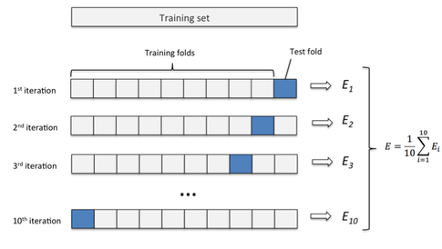
Keeping a fixed set of data points for validation might not be conducive for models like XGB. Hence, a k-fold validation is used. In a k-fold method, the entire dataset is divided into k folds. One of the fold is used for validation and the others are used for training. The final performance metric is the average of the metric of each fold.
Usually, the number of folds is taken to be 10.
The following illustration better explains a 10-fold cross validation.

26 Feb 2017
Decision Trees are one of the most intuitive models in the world of perplexing and obscure ML models. This is because of the similarity in the human decision making process and a decision tree.
A decision tree can be visualized and we can actually see how a computer arrived at a decision, which is rather difficult in case of other models. Hence, it is also called as a white box model.
The purpose of this post is to explore some of the intuition behind building a stand alone decision tree and it's ensemble variants, \( Random Forests (RF) \) and \( Extreme Gradient Boosting (XGB) \).
Decision Trees:
What is a Decision Tree?
A decision tree is a tree in which each node denotes a decision and the corresponding path to take depending on the decision made.
Decision trees are versatile and are widely used for both classification and regression models and are called CART (Classification and Regression Trees).
One of the main advantages of a decision tree is it's ability to handle missing data gracefully.
How is a decision tree built?
There are two metrics on which a decision tree is built, \( Information Gain \) and \( Standard Deviation \). Information gain is used to build a classification tree and standard deviation is used to build a regression tree.
In this post, I will be using a regression tree as an example.
- Decision tree is built in a top down approach.
- The goal of a tree is to partition the data into subsets such that each subset contains homogeneous values (with same target classes in case of classification and with minimum standard deviation in case of regression).
$$S(T) = \sqrt{\frac{\sum (x-\mu )^{2}}{N}}\; \mu\rightarrow mean$$
$$Entropy\; H(X) = -\sum p(X)\log p(X)\\ Information\ Gain\; I(X,Y)= H(X)-H(X|Y)$$
- In case of regression, if the sample is homogeneous i.e equal valued, standard deviation is 0.
- In case of regression, the goal is to decrease the standard deviation after the data is split into subsets. Hence, the attribute that can provide the highest decrease in standard deviation is chosen.
- In case of classification, the attribute that can provide the highest information gain is chosen.
- In simple words, a decision tree can be viewed as a decision table. If the tree is allowed to grow till the last depth, each leaf node will have only one sample. If the training data has all possible permutations of the independent variables, the decision tree becomes a representation of a truth table.
High level steps in building a regression tree are as follows:
- Step 1: Calculate the standard deviation of the target (dependant) variable \( S(T) \).
- Step 2:
- Split the data on all the attributes \( (X) \).
- Calculate the standard deviation of the subsets \( S(T,X) \).
- Choose the attribute with the highest difference.
- \( SDR(T,X) = S(T) - S(T,X) \)
- Step 3: Split the data according to the decision attribute selected in the previous step.
- Step 4: Repeat the process recursively.
- Step 5: We can repeat the process recursively until each subset of the data has 0 standard deviation. This is not feasible at a large scale and it represents a model with very high variation. Hence, we need a termination criteria. For example, the termination criteria could be that the standard deviation at each leaf node must be lesser than 5% or that each node must contain a minimum number of data points.
- Step 6: When the number of data points at a leaf node is more than one, the average of the target variable is taken as the output at that node.
How does a decision tree handle missing data?
During the process of building a tree, at each decision node, a decision is made for the missing data. All the data points with the missing data is first clubbed with the left subtree and the drop in standard deviation is calculated. The same is done by combining the missing data points with the right subtree. The branch with the highest drop in standard deviation is assigned to be the path to be followed for missing data points.
What are ensembles and why do we need them?
Ensembles are a combination of various learning models which is practically observed to provide a better performance than stand alone la carte models. This practise is also called as bagging.
One of the main disadvantage of a stand alone model, like a decision tree,which is addressed by an ensemble, is that they are prone to over fitting (high variance). Ensembles are used to average out the noisy data and unbiased (or low biased) models and to create a low variance model.
Two such ensembles for decision trees are Random Forest and XGBoost.
The fundamental issue that both RF and XGB try to address is that decision trees are weak learners (prone to over fitting and depends heavily on the training distribution). Hence, by combining a number of weak learners, we can build a strong learner.
- RF consists of a large number of decorrelated decision trees.
- Given a training data set, we create a number of subsets randomly. These subsets can be based on random selection of data or features (variables). These subsets can be overlapping.
- Build a decision tree for each of these subsets.
- In order to get a classification from a RF, the output from each tree can be polled in order to arrive at the decision.
- There can be a number of polling mechanisms, the most common being, the target variable with the highest frequency is chosen i.e the decision arrived to by the majority of the trees. We can also use a weighted average, where certain trees are given more weight-age than others.
Another variant of RF is called as XGBoost, which uses gradient boosting in order to build the trees. XGB models are used in cases where the data contains high collinearity. This is called as multicollinearity, where two or more features are highly correlated and one can be predicted with reasonable accuracy given the other.
Unlike RF, where the trees are built parallelly with no correlation between the trees, XGB model builds the trees sequentially (and hence, computationally expensive). It learns from each tree and builds the subsequent tree so that the model can better learn the distribution of the target variable i.e the errors are propagated from one tree to the other.
How are these models validated?
RF models are usually validated using Out-Of-Bag (OOB) validation and the XGB models are validated using k-Fold cross validation, which is explored in another post.
Given the simplicity and the intuitive nature of these models, they are one of the most widely used models for competitive ML like Kaggle. In fact, XGBoost models have won 65% of the competitions on Kaggle.
23 Feb 2017
It is officially declared that the process of awarding H1B visas by the government of US is based on a lottery system i.e a random process.
Therefore, as a random project, I decided to cross verify the claim. Is it truly random or is there a pattern underlying that is not apparent?
The US government releases the data of all applications for H1B and the status of whether they were certified or not. You can find the data at
United States Department of Labour.
I built a neural network in order to model this problem, where the features considered were:
- VISA_CLASS
- EMPLOYER_NAME
- SOC_NAME
- NAIC_CODE
- PREVAILING_WAGE
- PW_UNIT_OF_PAY
- H1-B_DEPENDANT
- WILLFUL_VIOLATOR
- WORKSITE_STATE
There were around 647000 data points for 2016 alone, with the target classes being
- CERTIFIED
- CERTIFIED_WITHDRAWN
- WITHDRAWN
- DENIED
Initially, I was getting around 94% accuracy in the first epoch itself. I realised that I failed to understand the data and to build a baseline model first. You can read about the importance of building a baseline model in my blog post here,
Importance of Baseline Models.
The data suggested that 89% of the 647000 data points were falling under the 'DENIED' category. The baseline model itself was giving me 89%. Hence, it was no wonder that the model was showing such high accuracies.
In order to handle such a skewed dataset, I decided to create my own dataset with the following distributions:
- CERTIFIED - 40%
- CERTIFIED_WITHDRAWN - 20%
- WITHDRAWN - 20%
- DENIED - 20%
From this distribution, we can clearly see that the baseline accuracy should be 40%. Due to the limitations on my personal computer, I was able to take only 50000 data points for training. The performance of the model was 61%. A bump in 21% accuracy is nothing to be ignored. At the same time, it does not conclusively prove that the process of awarding H1B visas has any underlying pattern.
I have some more modifications in mind, that I believe would improve the model and can point to some conclusion. I will update this post once I am done with that.
Also, using at least 80% of the data set for training might throw some new light on the pattern. Also, considering more features might help better the model. This would require significant computing power. This would enable us to build a more complicated and deeper neural network that might be able to capture the underlying pattern, if any.
But for now,it seems that there is nothing that can be said about the randomness of H1B visas.
23 Feb 2017
One of the important aspects of building a machine learning model is to understand the data first. Most of us forget this and jump right into modelling. Another corollary to this is that we often times forget to build a baseline model before building something complicated.
What is a Baseline Model and a Baseline Accuracy?
A baseline model, in simple words, is the most simple model that you can build over the provided data. The accuracy that is achieved by a baseline model is the lower bound for evaluating the performance of your model.
A baseline model usually does not include any machine learning approaches, rather a statistical approach. It also include heuristics, randomness or simple statistics in order to come up with a value.
Sklearn supports baseline models in the form of
Dummy Classifiers:
- “stratified”: generates predictions by respecting the training set’s class distribution.
- “most_frequent”: always predicts the most frequent label in the training set.
- “prior”: always predicts the class that maximizes the class prior.
- “uniform”: generates predictions uniformly at random.
- “constant”: always predicts a constant label that is provided by the user. This is useful for metrics that evaluate a non-majority class.
In the case of regression, a baseline model could be any of the following:
- Median or average
- Constant
Ideally, the performance of the machine learning model should be much greater than the statistical performance.
In case of models that are already implemented, we can use the performance of the existing models as a frame of reference and they become baseline models.