
Exploring Word2Vec
03 Mar 2017 In my previous blog post, I explored some of the early ways of word embeddings and their shortcomings. The purpose of this post is to explore one of the most widely used word representations in the natural language processing industry today.Word2Vec was created by a team of researchers led by Tomas Mikolov at Google. According to Wikipedia,
Word2vec is a group of related models that are used to produce word embeddings. These models are shallow, two-layer neural networks that are trained to reconstruct linguistic contexts of words. Word2vec takes as its input a large corpus of text and produces a vector space, typically of several hundred dimensions, with each unique word in the corpus being assigned a corresponding vector in the space. Word vectors are positioned in the vector space such that words that share common contexts in the corpus are located in close proximity to one another in the space.There are many resources on the internet providing a detailed mathematical explanation and derivations of Word2Vec and the reason why they perform so well. I have included links to some of them at the end of this post. The purpose of this post is to explore Word2Vec in a graphical manner in order to get an intuitive feel of how Word2Vec works, what the vectors mean and why they perform so well.
Let us look at the equation proposed by Mikolov,

As we can see from the equation, it is nothing but a softmax equation.
Intuitively, we can visualize the model as follows. The main operation being performed here is that of dimensionality reduction. We have seen the usage of neural networks for dimensionality reduction in auto-encoders. In auto-encoders, we trick the neural network to learn compressed representations of vectors by providing the same vector as both input and target. In this way, the neural network learns to reproduce a vector from a compressed representation. Hence, we can replace the high dimension input vectors by their lower dimension hidden activations (Or weight matrices).
Similarly, in Word2Vec we trick the "neural net" to learn smaller dimensions representations of the huge dimensioned one hot vector.
But unlike in auto-encoders, we do not provide the same vector as both target and input vector. Although this can be used to reduce dimensions, we need to capture the syntactic and semantic meaning of every word. In order to accomplish that, we need to consider a window of words around the current word (context). How do we add this context to the representation of the current word? We make the neural net predict the current word given its context (CBOW) or to predict the context given the current word (Skip Gram).
Once the neural net is trained to predict a word given it's context, we are going to strip off the hidden-output connections (just like auto-encoders) and use the trained weight matrix between input and hidden as vector representations (just like auto-encoders)
Graphically, the model can be visualized as follows:

V - Vocabulary Size
H - Size of Word2Vec vector
There is a distinct difference between the above model and a normal feed forward neural network. The hidden layer in Word2Vec are linear neurons i.e there is no activation function applied on the hidden activations.
Also, we can see that the dimensions of input layer and the output layer is equal to the vocabulary size. The hidden layer dimension is the size of the vector which represents a word (which is a tunable hyper-parameter).
Now, let us take an example in order to understand this better and we'll go through each layer separately.
"The night is darkest just before the dawn rises"From the above corpus we can see that the vocabulary size is 8.
For simplicity, let us make the following assumptions:
Window size = 1
Word2Vec dimension = 3
The initial one-hot representations will be
The - [1,0,0,0,0,0,0,0]
night - [0,1,0,0,0,0,0,0]
is - [0,0,1,0,0,0,0,0]
darkest - [0,0,0,1,0,0,0,0]
just - [0,0,0,0,1,0,0,0]
before - [0,0,0,0,0,1,0,0]
dawn - [0,0,0,0,0,0,1,0]
rises - [0,0,0,0,0,0,0,1]
Let us consider the following scenario, where the current word is darkest and the context word is just. Let us assume that this is a Continuous Bag Of Words (CBOW) model where we predict the current word given the context words.
Input Layer:
Word: just
Vector: [0,0,0,0,1,0,0,0]
Hidden Layer:
Dimension = 3
Winput-hidden is of dimension 8X3
Whidden-output is of dimension 3X8
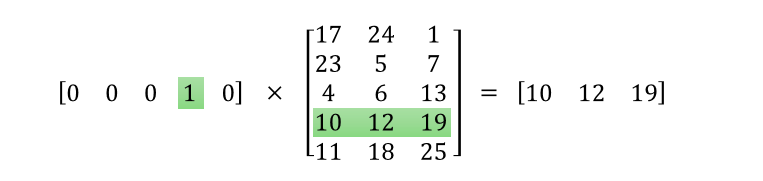
Since the input is a one-hot vector, the hidden activation is just a lookup operation. That is, hidden activation just looks up the row corresponding to the word ID in Winput-hidden and passes it on to the output layer. As an illustration,
Output Layer:
Target word - darkest [0,0,0,1,0,0,0,0]
Since the output layer is a softmax layer, it produces a probability distribution across the words. Thus, the categorical logloss is calculated (and since this is a softmax, the error is just the difference between the target vector and the output vector). This error is then back propagated to the hidden layer.
As you might have noticed, this procedure gives us two trained parameters. The Winput-hidden and Whidden-output. Usually, Whidden-output is discarded.
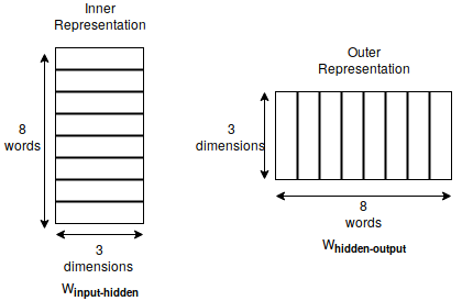
In the Mikolov's equation we saw above, Vw is the inner representation of the word i.e from Winput-hidden and VIw is the outer representation of the word i.e from Whidden-output.
Inner representation is nothing but the representation of the word when it is the current word and outer representation is when the word occurs in the window of another word.
After the training process, the Winput-hidden is just a lookup table, given the index, it returns the 3 bit inner representation of the word. Similarly, Whidden-output is a lookup table for the outer representation of the word.
Why does this work?
This method accomplishes dual task of reducing the dimensionality and adding semantic meaning to the word. How?
Let us take 2 pairs of words. ('Computers', 'ML') and ('NFL', 'Kobe'). If we look at the above pairs, we can see that 'Computers' and 'ML' occur in the same context in the corpus. Hence, the representations of the words 'Computers' and 'ML' will be very close to each other (cosine similarity). Whereas, there is no way 'NFL' would be a part of a discussion about 'ML' (Although there is a Kobe challenge on Kaggle, which we are assuming is absent from the corpus) and hence the similarity between them will be very low. Since the context will be similar to 'Computer' and 'ML' and 'NFL' and 'Kobe', the neural net is forced to learn similar representations for each of these pairs.
This also handles stemming on a certain level, as 'Computers' and 'Computer' occur in the same context and can be interchanged. This also has the ability to handle acronyms. Since 'ML' and 'Machine' and 'Learning' occur in the same contexts, all 3 words will have similar representations.
One important thing to note is that Word2Vec does not consider the positional variable of the context words i.e whether the word 'Learning' comes before 'Machine' or after is immaterial to the model. It does not learn a different vector for 'Learning' when it occurs before 'Machine' or after.
Here are some of the resources where you can find the detailed mathematical derivation for Word2Vec:
http://www.1-4-5.net/~dmm/ml/how_does_word2vec_work.pdf
http://www-personal.umich.edu/~ronxin/pdf/w2vexp.pdf
https://cs224d.stanford.edu/lectures/CS224d-Lecture2.pdf