Audio and Speech Signal Processing (ASR Part 1)

04 Dec 2018

Link to the start of ASR series: Automatic Speech Recognition (ASR Part 0)

Input to the ASR system will be an audio file/stream that encodes the speech. How this speech is stored, transmitted and encoded is explored in this post.

How humans produce and perceive speech is vastly different from how we intuitively try to understand speech. Speech consists of multiple deterministic signals interspersed within indeterministic boundaries.

Human Ear

Human ear can perceive sounds with frequencies in the range \(20Hz\) to \(20kHz\). But this is not linear i.e we are more sensitive to lower frequencies than higher frequencies. For eg, we can perceive the difference between a signal at \(1kHz\) and a signal at \(2kHz\) better than \(19kHz\) and \(20kHz\). This range is dependent on the individual and age. This is why we use a logarithmic filterbank (called Mel filterbank). In this filterbank, the filters become wider and longer as the frequency increases. Mel filterbank of length 40 is typical. i.e 40 filters. It is represented as a matrix where each row is a filter.

Broad overview of audio pre-processing to accommodate human ear limitations:

Conversion to frequency domain (Fourier transform - we use only magnitude and not phase) -> Mel filterbank filtering -> Logarithmic compression (Again because of human ears).

Audio and Signals

When a sound is produced, it creates pressure differences in air (sound waves). These pressure differences are responsible for the to-fro movements of the magnet in the coil of the microphone and this in turn generates current/speech signals. These signals that are generated and transmitted over the wire can be visually demonstrated using a waveform.

How do we store these speech signals in a computer? Let us assume that we are storing it in 32 bit. This means that this alternating current (in ampere) will be converted to a number (positive/negative). For 32 bits, the max positive number it can store is \(x\) (let’s say) and max negative number it can store is \(-x\). So the current will be converted to a series of numbers that is represented as a 32 bit float.

Usually speech signals are stored in 32 bit. It can also be stored in 16 bit, 64 bit etc. The visual representation of this can be seen in a waveform.

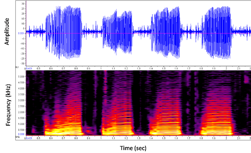
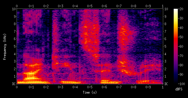
In the previous step, we have amplitude on \(y\) axis and time on \(x\) axis. Now we need to convert it into the frequency scale (called spectrogram). For this, we first take a small piece of time segment (called frame) from the previous step and convert it into a frequency representation. Here, on \(x\) axis we get the series of frames that we’ve sampled. On \(y\) axis, we get the distribution over all frequencies (Like a softmax at each frame step).

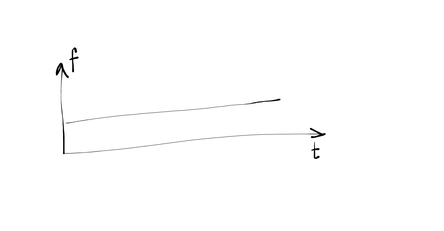
For eg, let us say that the frame we sampled has a \(sine\) curve and that this \(sine\) function has a frequency \(f\) (which is fixed). Therefore, for this frame there will be a single peak at the frequency \(f\) and 0 everywhere else. If the entire waveform is the same \(sine\) graph (i.e every frame in the waveform has the same curve), in each frequency distribution, there will be the same single peak at \(f\). This will result in a horizontal line (just like a softmax).

In this frequency distribution, the max frequency it can take is a specification. Phones usually do \(8kHz\). ASRs like Kaldi and CMUSphinx need recordings at or above \(16kHz\). Normally we record in \(44kHz\) for music.

Sample Numbers:

While converting the audio signal from amplitude domain to the frequency domain, we spoke about taking small time segments called frames (called sampling-rate). If the audio that we have is a \(16kHz\) audio, we have \(16 \times 10^{3}\) numbers for each \(1 s\). Usually, the window size for sampling is \(25 ms\) with a \(10 ms\) step. Hence, each frame size will be \(16 \times 10^{3} \times 25 \times 10^{-3} = 400\). Hence, we will get a vector of size \(400\) every \(10 ms\).

Overview of audio processing

• Dithering: Adding a very small amount of noise to the signal to prevent mathematical issues during feature computation (in particular, taking the logarithm of 0).
• DC-Removal: Removing any constant offset from the waveform.
• Pre-emphasis Filter: Applying a high pass filter to the signal prior to feature extraction to counteract that fact that typically the voiced speech at the lower frequencies has much high energy than the unvoiced speech at high frequencies.
• Mel Filtering: Binning and applying the filter on each frame.
• Log of Mel Frequencies: Taking log of the values from previous step.

At the end of these steps, we get vectors called as MFCC (Mel-frequency cepstral coefficients) vectors which are then used as the representation of the audio. We can think of these MFCC vectors as analogous to word embeddings in the NLP domain.

Cepstral Mean and Variance Normalization (CMVN)

As soon as we dive into any ASR system, we will be accosted with the term CMVN in the pre-processing step right after MFCC generation. It is important to understand the significance of this normalization step and to do that, we need to understand what it is.

Whenever a signal (audio in our case) passes through a noisy channel, the channel introduces some noise to the signal. This is referred to as channel impulse response in signal processing lingo. Whenever an impulse signal is sent through a channel, the channel distorts this impulse in a certain way.

When we record any audio with voice, it consists of the pure voice signal \(x[n]\) and the channel impulse response \(h[n]\). Therefore, the recorded signal is a linear convolution of both of them and is given by,

\[y[n] = x[n] \bigstar h[n]\]

When we take the Fourier Transform of the above signal (which we do to get MFCC), linear convolution becomes simple product.

\[Y[f] = X[f].H[f]\]

Further, in the process of calculating MFCC, we take the logarithm of this value and we end up with,

\[Y[q] = log(Y[f]) = log(X[f].H[f]) = X[q]+H[q]\]

since \(log(a.b) = log(a)+log(b)\).

We can see that any linear convolution distortion in the audio is represented as an addition in the cepstral domain. Let us assume that the channel impulse response is constant for a given channel (This is a strong assumption since we are assuming that the noise component of the channel is going to remain stationary). Then, for a series of audio signals,

\[Y_{i}[q] = X_{i}[q] + H[q]\]

By taking average of all the frames,

\[\frac{1}{N}\sum_{i}Y_{i}[q] = H[q]+\frac{1}{N}\sum_{i}X_{i}[q]\]

If we subtract this mean from each cepstral coefficient, we get,

\[R_{i}[q]=Y_{i}[q]-\frac{1}{N}\sum_{j}Y_{j}[q]\] \[R_{i}[q]=X_{i}[q] + H[q] - \left ( H[q]+\frac{1}{N}\sum_{j}X_{j}[q] \right )\] \[R_{i}[q]=X_{i}[q] - \frac{1}{N}\sum_{j}X_{j}[q]\]

In the above equation, we can see that the channel effects (distortions) are removed. In simpler words, subtracting the mean from all cepstral coefficients (such that the mean of all vectors is zero) (this process is called CMVN) removes the channel distortions from the signal and hence is an important pre-processing step in speech recognition.