30 Jun 2018
Word embeddings are the staple of any Natural Language Processing (NLP) task. In fact, representation of words in the form of vectors is probably the first step in building any NLP application. These vector representations of words fall in a wide spectrum in semantic encoding space, with a one-hot representation on one end of the spectrum, encoding absolutely nothing in terms of semantics between words and the other end of the spectrum still being an active area of research with ELMo embeddings achieving state of the art results. Most widely used embeddings such as Word2Vec and GloVe fall somewhere in between on this spectrum.
Although these word embeddings encode semantic relationships between words and can be efficiently used as vector representations of words, these embeddings cannot directly be applied to NLP tasks. Majority of NLP tasks deal in sentences and paragraphs (a set of words, to be more formal) and not individual words themselves. Therefore, there is a need for efficient semantic embeddings for groups of words, henceforth referred to as sentence embeddings.
Averaging of individual Word2Vec embeddings is one of the most widely used sentence embedding techniques. Although it might sound naive, hey, it works. There definitely exists some information loss when we average out word2vec vectors which get cancelled out when another learning algorithm is stacked after the averaging operation.
Another approach to sentence embedding is to treat the words in a sentence as sequence inputs at respective time steps. Hence, it can be modeled using a recurrent neural network architecture where the each word is treated as input at current time step. The encoded representation or the last hidden state activation at the final time step is taken as the sentence embedding.
One of the most recent research in sentence encoding comes from Google, which has open sourced their implementation in the form of Universal Sentence Encoder. Universal Sentence Encoder is an implementation of two sentence encoding architectures, Deep Averaged Networks and Transformer.
Deep Averaged Network is a simple feed forward neural network that takes the average of word embeddings as the input layer, stacks two hidden layers and culminates with a softmax over the target classification. The last hidden layer activation is taken as the sentence embedding.
The Transformer architecture is a variant of recurrent neural network, where a convolution is implemented over the input sentence. Each word is embedded using an existing word embedding technique with an additional positional embedding. These word embeddings are passed through a convolutional layer with attention mechanism. The decoder stage generates the context/future words given a sequence of words. The hidden state activation is taken as the sentence embedding.
While these approaches are promising, employing complex neural architectures fail to perform significantly better than simple old-fashioned averaging of word vectors. In most of the NLP tasks, instead of employing such complicated architectures in your model, you will be better off employing simple average based sentence encodings and optimizing your classification model.
Since we have decided to go down the averaging route, we can explore different kinds of averaging in order to better embed sentences. One of the approaches is to employ tf-idf weighted average of word vectors instead of a simple average, which in practice turns out to be an embarrassingly good sentence embedding. Any averaging technique is dependent on the quality of the underlying word embeddings. Therefore, any improvement in word embeddings has a direct effect on sentence embeddings. This is where ELMo embeddings come into the picture.
ELMo (Em-beddings from Language Models) is a word representation algorithm that is providing state of the art results in downstream NLP tasks. They are presented in the following paper: Deep Contextualized Word Representations. The architecture consists of 1 word embedding layer and 2 hidden bi-LSTM layers, for both forward and backward representations. ELMo is modeled on image classification neural network ResNet and hence, the defining characteristic of ELMo is that it exposes the hidden layer activations for each word. A weighted average of these activations yield the word embedding. These weights are learnable parameters and can be fine tuned for the NLP task at hand. Since the entire ELMo model is pre trained on big corpus and only these weights are learned for the task at hand, it falls into transfer learning territory and is best suited for any NLP task with less amount of data.
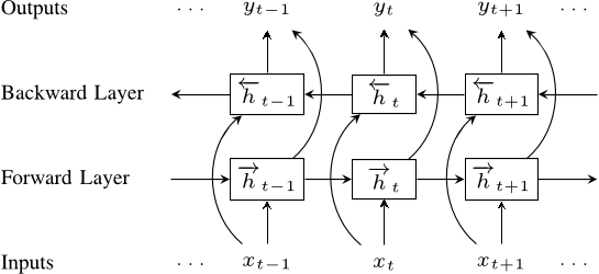
One important point about the above architecture is that, ELMo takes words as input character wise. A 2048 character n gram convolutional filter is applied on the characters of the words, followed by a projection on the 512 dimension vector space for each word. This gives ELMo the ability to handle unseen words and even commonly miss-spelt words.
Assume that ( t_{k} ) is the current word (token) that needs to be embedded, the following probabilities is modeled by the forward and backward LSTM layers:
\[p(t_{1},t_{2},...,t_{N}) = \prod_{k=1}^{N}p(t_{k}|t_{1},t_{2},...,t_{k-1})\]
\[p(t_{1},t_{2},...,t_{N}) = \prod_{k=1}^{N}p(t_{k}|t_{k+1},t_{k+2},...,t_{N})\]
Given the token ( t_{k} ) (word), the convolutional filter is applied on the characters and projected into the word embedding space. This projection is denoted by ( x_{k} ).
If the architecture consists of ( L ) hidden layers, for the token ( t_{k} ), we get ( 2L ) hidden representations (forward and backward) and 1 word embedding representation ( x_{k} ), which can be represented as:
\[R_{k} = \{x_{k}, h_{k,j}^{forward}, h_{k,j}^{backward} | j=1,2,...,N\}\]
Concatenating the forward and backward representations, each token ( t_{k} ) has ( 2L+1 ) representations, which can expressed as:
\[R_{k} = \{h_{k,j} | j=0,1,2,...,N\}, where \quad h_{0,j}=x_{k}\]
Now, the ELMo representation of this word (which is task dependent) is expressed as:
\[ELMo_{k}^{task} = \gamma^{task}\sum_{j=0}^{L}s_{j}^{task}h_{k,j}\]
where \(\gamma^{task}\) is a scaling parameter.
Both \(\gamma^{task}\) and \(s_{j}^{task}\) are learnable parameters that are trained specific to the NLP task at hand.
16 May 2018
Conditional Random Field (CRF) is the go-to algorithm for sequence labeling problems. Initial attempts at sequence labeling such as POS tagging and Named Entity Recognition were accomplished using the Hidden Markov Models. Although HMMs gave promising results for the same, they suffered from the same drawbacks as using a Naive Bayes models i.e conditional independence.
Both Naive Bayes (and HMM in extension) try to fit a model that maximizes the joint probability distribution \( P(X , Y) \). This is flawed on two levels. One, since \( X \) is already given, trying to fit a joint distribution over both \( X \) and \( Y \) is computationally expensive, wasteful and in the end, we do not require the type of distribution the input variable follow. We just need to know what distribution the target variable follows given an input variable. Second, since we are assuming that the input variables are conditionally independent, if there exists some correlation between the variables, the model assigns high probability when these two variables occur together instead of generalizing over the input distribution. Hence, we can see that any perturbance in the input distribution has a significant effect over the output. Ideally, since we only care about the distribution of the target variable \( Y \), this should not be under consideration. We should evaluate \( P(Y | X) \) instead of \( P(X , Y) \).
In hindsight, this might seem trivial and as the obvious choice for any classification problem. In fact, majority of the classifiers in use today optimize over this metric. Nevertheless, it was an important breakthrough when it was considered decades ago.
A Conditional Random Field (CRF) does exactly this. It evaluates \( P(Y | X) \). The purpose of this post is to delve deeper into the mathematics of a CRF and why CRF is considered to be the starting point for most of the current classification algorithms.
Consider a function \( Q(.) \) as a real valued function. According to Markovian distribution theorem,
$$P(X,Y) \propto exp(\sum _{c\in C}Q(c, X,Y))$$
Where \( C \) is a set of feature verticals (or cliques). This equation provides us with the un-normalized joint probability distribution over \( X \) and \( Y \). Since we are interested in calculating the conditional probability,
$$P(Y|X)= \frac{exp(\sum _{c\in C}Q(c, X,Y))}{\sum _{X}exp(\sum _{c\in C}Q(c, X,Y))}$$
This is similar to Gibbs Distribution (or Softmax depending on the \( Q(.) \) function). The above equation can be re written as
$$P(Y|X)= \frac{\prod _{C}\phi _{C}(X, Y)}{Z}$$
Where \( \phi _{C}(X, Y) = exp(Q(C,X,Y)) \) and \( Z \) is called as the Partition Function.
$$Z = \sum _{X}exp(\sum _{c\in C}Q(c, X,Y))$$
For a CRF which is used for sequence labelling such as PoS or NER, the graph forms a linear chain and the probability equation can be written as
$$P(Y_{1},Y_{2},...,Y_{M}|X) = \frac{1}{Z}\prod _{i}\phi (Y_{i},X)\phi^{1}(Y_{i-1},Y_{i},X)$$
Where, \( \phi () = exp(\sum _{k}\theta _{k}s_{k}(y_{i},x_{i},i)) \) and \( \phi^{1} () = exp(\sum _{j}\lambda_{j}t_{j}(y_{i-1},y_{i},x_{i},i)) \).
\( s_{k} \) is the state feature function and \( t_{j} \) is the transition feature function (Similar to HMMs).
CRF is a generalized method of calculating \( P(Y | X) \) and is not restricted to just evaluating sequence label probabilities. The flexibility of CRFs stems from the ability to choose any function as \( Q(X , Y) \). In the following section, we can see how the logistic function can also be derived from CRF.
Consider the feature function,
$$\phi (X_{i},Y) = exp(w_{i}1(X_{i},Y))$$
where \( 1 \) is an indicator function. It can also be denoted as
$$\phi (X_{i},Y) = exp(w_{i}* AND(X_{i},Y))$$
Calculating the probabilities,
$$\phi (X_{i},Y=1) = exp(w_{i}X_{i})$$
$$\phi (X_{i},Y=0) = exp(0)=1$$
Therefore, substituting the above results in the CRF equation, we get,
$$P(Y|X) = \frac{\phi (X_{i},Y=0) * \phi (X_{i},Y=1)}{\phi (X_{i},Y=0) + \phi (X_{i},Y=1)} = \frac{exp(\sum _{i}w_{i}X_{i})}{1+exp(\sum _{i}w_{i}X_{i})}$$
The above equation is nothing but the logistic equation. Hence, we can see that CRF is a generalized form of any machine learning classification problem.
27 Jan 2018
We are fully aware of the marked influence of the introduction of Word2Vec method of word embedding on the Natural Language Processing domain. It was a huge leap forward from the hitherto constricting method of word embeddings namely, Term Frequency (TF) and Inverse Document Frequency (IDF). Neither of these methods were anywhere close to preserving the semantics of the words in their representations. With the introduction of Word2Vec and the possibility of semantic embedding in the vectors, various avenues were thrown open where this representation could be exploited for various NLP applications.
One of the logical extensions to Word2Vec was document similarity. Now that you could find out similarity between words, what was the best way of classifying or clustering documents semantically? There are two metrics by which we can quantify the similarity between two words, cosine similarity and Euclidean distance.
Word Mover's Distance (WMD) was introduced in 2015 which leveraged Euclidean distance in order to quantify similarity between documents. WMD accomplishes this by quantifying the amount of distance that the embedded vectors in a document needs to travel in order to match the embedded vectors in another document, thereby offering us a proxy which quantifies dissimilarity (or similarity) between two documents. You can find a link to the original paper
here.
For example, let us consider three documents,
D1: "
Obama speaks to the media in Illinois"
D2: "
The President greets the press in Chicago"
D3: "
Obama speaks in Illinois"
WMD algorithm can be described in the following steps.
- Each word in a sentence can be represented as a point in the \( (n-1) \) dimensional simplex of word distribution. The magnitude of the vector is represented by it's nBOW (n Bag Of Words) representation. Mathematically, if the word \( i \) appears \( c_{i} \) times it can represented as,
$$d_{i} = \frac{c_{i}}{\sum_{j=1}^{n}c_{j}}$$
where \( i \) is a vector in \( n \) dimensional space specified by vocabulary size. It is perfectly clear from the above description that each word pair, if they are dissimilar, lie in a completely different plane irrespective of their semantic distance.
- In the example considered above, after stop words removal, the nBOW representations of documents D1 and D2 have zero common non zero elements and hence lie in the max distance possible from each other even though semantically these sentences are close.
- The distance metric used between any word pair is given by the Euclidean distance between the Word2Vec vectors. We will denote this distance between the word \( i \) and word \( j \) as \( c(i , j) = || x_{i} - x{j} || \), where \( c(i , j) \) is the traveling cost from word \( i \) to word \( j \).
- The objective of the WMD algorithm is to calculate the flow matrix \( T \). Flow matrix \( T \) can be defined as a sparse matrix of dimension \( n X n \).
$$T \in R^{n X n} \hspace{0.2cm}where \hspace{0.2cm} T_{i,j}\geq 0$$
In the flow matrix \( T \), \( T_{i,j} \) denotes how much of word \( i \) in \( d \) flows into word \( j \) in \( d' \). Naturally, the sum of the outgoing flow from word \( i \) should be equal to \( d_{i} \) and the sum of the incoming flow to word \( j \) should be equal to \( d'_{j} \). Mathematically,
$$\sum_{j} T_{i,j} = d_{i}$$
$$\sum_{i} T_{i,j} = d'_{j}$$
- Finally, we can calculate the distance between the two documents \( d \) and \( d' \) by calculating the minimum cumulative cost required to move all words in \( d \) to \( d'\).
$$\sum_{i,j} T_{i,j}c(i,j)$$
- The minimum cumulative cost can be formalized with constraints as follows,
$$\underset{T\geq 0}{min}\sum_{i,j} T_{i,j}c(i,j)$$
subject to \( \sum_{j} T_{i,j} = d_{i} \) and \( \sum_{i} T_{i,j} = d'_{j} \)
- The solution to the above problem is a variation of the Transportation Problem called Earth Mover's Distance which can be found here.
Although the algorithm seems simple enough when the number of words in the 2 documents are equal, complications arise when the number of words are different, as in the case between D2 and D3. In that case, the computational complexity increases to \( O(P^{4}) \). Hence, this algorithm is computationally very expensive.
06 Dec 2017
Hidden Markov Models (HMM) were the mainstay of generative models a couple of years ago. Even though more sophisticated Deep Learning generative models have emerged, we cannot rule out the effectiveness of the humble HMM. After all, one of the most widely known principle (Occam’s Razor** states that if you have a number of competing hypothesis, the simplest one is the best one. The purpose of this blog post is to explore the mathematical basis on which HMMs are built.
Hidden Markov Models are characterized by two types of states, Hidden States and Observable States. Any HMM can be represented by three parameters:
Transition Probability:
The probability of the model to transition from one hidden state to the other given the current state.
Emission Probability:
The probability of the model to emit an observable state given the current hidden state.
Initial Probability:
The probability of the model being in a specific hidden state when it starts off.
Graphically, HMM are represented using a Trellis Diagram:
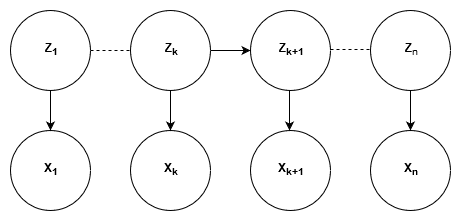
There are four algorithms fundamental to HMM: Forward algorithm, Backward algorithm, Forward-Backward algorithm and Viterbi Algorithm.
Forward Algorithm: Goal - To calculate \(P(Z_{k},X_{1:k})\)
Using marginalization,
\[\sum_{Z_{k-1}}^{n}P(Z_{k},Z_{k-1},X_{1:k})\]
\[\sum_{Z_{k-1}}^{n}P(X_{k},X_{1:k-1},Z_{k},Z_{k-1})\]
\[\sum_{Z_{k-1}}^{n}P(X_{k}|X_{1:k-1},Z_{k},Z_{k-1})P(Z_{k}|Z_{k-1},X_{1:k-1})P(Z_{k-1},X_{1:k-1})\]
Since \(X_{k}\), \(X_{1:k-1}\) and \(Z_{k-1}\) are independent,
\[\sum_{Z_{k-1}}^{n}P(X_{k}|Z_{k})P(Z_{k}|Z_{k-1})P(Z_{k-1},X_{1:k-1})\]
\[\alpha_{k} = \sum_{Z_{k-1}=1}^{n}(Emission Probability)(Transition Probability)\alpha_{k-1}\]
Backward Algorithm: Goal - To calculate \(P(X_{k+1:n}\|Z_{k})\)
Using marginalization,
\[\sum_{Z_{k+1}=1}^{n}P(X_{k+1}, X_{k+2:n}, Z_{k+1}| Z_{k})\]
\[\sum_{Z_{k+1}=1}^{n}P(X_{k+1}| X_{k+2:n}, Z_{k+1}, Z_{k})P(X_{k+2:n}| Z_{k+1}, Z_{k})P(Z_{k+1}| Z_{k})\]
\[\sum_{Z_{k+1}=1}^{n}P(X_{k+1}| Z_{k+1})P(X_{k+2:n}| Z_{k+1})P(Z_{k+1}| Z_{k})\]
\[\beta _{k} = \sum_{Z_{k+1}=1}^{n}(Emission Probability)\beta_{k+1}(Transition Probability)\]
Forward-Backward (Baum Welch) Algorithm: Goal - To calculate \(P(Z_{k}\|X)\)
where \(X = (X_{1}, X_{2},.. X_{n})\) and \(P(Z_{k}|X)\propto P(Z_{k},X) = P(X_{k+1:n}|Z_{k},X_{1:k})P(Z_{k},X_{1:k})\)
Here, \(X_{k+1:n}\) is independent of \(X_{1:k}\) given \(Z_{k}\)
\[P(Z_{k},X) = P(X_{k+1:n}|Z_{k})P(Z_{k},X_{1:k})\]
\[P(Z_{k},X) = (Backward Algorithm)(Forward Algorithm)\]
21 Jul 2017
I recently came across a
blog post by Francois Chollet, the creator of Keras, where he explores the limitations of deep learning methods. It is an extremely informative blog piece, which I would recommend readers to go through before continuing further.
I, personally, am guilty of over estimating the capabilities of deep learning for machine learning tasks. Theoretically, a recurrent neural network can be considered as a Turing Complete machine. To put it in a simpler phrase, every Turing Machine can be modeled by a recurrent neural network. In other words, any algorithm can be modeled using a recurrent neural network. Does this mean we don't need to learn algorithmic programming anymore and just throw enough sample training data to the neural net and let the net learn the algorithm? This is where the catch is. Neural networks are universal approximators. They can never leverage precision decision boundaries like an actual algorithm. They approximate the underlying function in order to produce outputs of varying precision. The phrase "varying precision" is of utmost importance since it can also represent a machine that is infinitely bad.
In order to comprehend why deep learning is over hyped and may not perform up to our expectations, we need to dive deeper into how a neural net does what it does. Like Francios rightly pointed out, we tend to think of a neural net as a replica of a human brain, both in terms of form and functionality. This can be attributed to the similar nomenclature used in these two contexts. For example, both the brains and the neural nets consists of neurons that are central to the decision making process, where different neurons get fired in response to different data points (stimuli, for brain). But this is where the similarity ends. Human neurons are much complex and have the ability to handle a diverse set of stimuli. Neural nets neurons on the other hand are simple differentiable functions which just applies a non linearity to the input data. Although the neural nets are modeled on human brains and are ideally expected to mimic its functionality, the status quo suggests that we are way too primitive to achieve such performance.
Deep learning methods are constrained in the geometric space. It is all about mapping one set of data in one vector space to another set of data in another vector space, one point at a time. There are two requisites for any deep learning model to perform well. One, availability of large (and by large, I mean very large) densely sampled, accurate data and the other is the existence of a learnable function. The requirement of a large set of training data is understood well by the public (thanks to the widespread media coverage). The other requirement of having a learnable function is more obscure and sometimes eludes the most seasoned deep learning engineer. This fact can be demonstrated by the below par performance of a neural net in as simple a task as sorting a list of numbers. Even after throwing millions of data points at it, it would still not perform well. Contrast this with the ability of a human brain to map the sorting function given a few examples.
This weakness of the neural nets has been brought to the forefront in recent times with importance being given to the adversarial examples, where the neural nets can be fooled completely by addition of a different overlay over the input image. Although the images looks identical to any human being, the neural net is unable to comprehend each of them. This highlights the fact that humans and neural nets comprehend an image in a completely contrasting manner. This should drive home the fact that we should never expect the neural net to perform like a human brain (at least not in the near future).
Francois also talks about Local and Extreme Generalizations. Deep learning methods are pretty good at local generalizations. They excel at mapping a narrow set of data points from one vector space to another vector space. When faced with a new data point far from the already encountered data points, the neural nets perform unpredictably. Human cognition, on the other hand, is adept at extreme generalizations, capable of applying cognition from one area into another seamlessly.
The status quo is such that, we are trying to model a bike cruiser using lego blocks with a motor attached. Although the intentions and the end goal is to have a cruiser, we cannot expect a lego model to replace it. Hence, we should be cautious while estimating the performance of any deep learning method.