25 Jun 2017
One of the major drawbacks of neural networks (or any machine learning model, in general) is the inability to handle data with huge dimensions, effectively. In this blog post, I will be exploring the technique of neural embedding, which is a variation on using auto-encoders for dimensionality reduction.
Data with high dimensions pose a very unique problem to any statistical analyses as the volume of the vector space under consideration increases exponentially with increase in dimensionality. As the vector space increases exponentially, the number of data points has to grow exponentially in order to retain the statistical significance of the data. Else, the sparsity of the data increases which hinders the statistical analysis employed by a majority of machine learning algorithms. This problem is usually referred to as the
Curse Of Dimensionality.
There are numerous approaches for dimensionality reduction, with Principal Component Analysis (PCA) and Auto-Encoders being the most widely used methods for linear and non linear reduction respectively.
Auto-Encoders are feed forward neural networks that are used to reduce the dimensions of the input vector and convert them from a sparse representation into a dense representation. The simplest of these encoders have a single hidden layer, consisting of neurons equal to the desired output dimensionality. The differentiating factor of auto-encoders from a normal feed forward neural network is that the target vector is the same as the input vector. The input-hidden weights are forced to learn the dense representations of sparse input vectors. The hidden-output weights are tuned in such a way that the dense representation can be used to reasonably recreate the input vector. Hence, the neural network is forced to reduce dimensions without losing information (much information, anyway). Thus, instead of using the high dimensioned input vector, feed it as input to the trained auto-encoder and use the hidden activation as the replacement for your machine learning applications. Auto-encoders can be as deep as you wish it to be. Sometimes, a single hidden layer is not enough to encode the input vector. In that case, we can have as many hidden layers as needed and the appropriate hidden layer activation can be considered as the dense representation of input vector.
A variation of this technique is employed in Word2Vec, a widely used word embedding technique (
Exploring Word2Vec). Since the target vector in auto-encoders are same as the input vector, each data point is considered independent of each other i.e it is assumed that there is no semantic relation between the data points. On the contrary, as we know, words are semantically linked to each other, more so with the neighbouring words. Hence, in the case of Word2Vec, if the input vector is a vector representation of the current word, the target vector is the vector representation of the neighbouring word. This ensures that along with the dimensionality reduction of the vector representation, the neural net also preserves the semantic relation between neighbouring words. A classic case of two birds, one stone.
We can further tweak the auto-encoders along the lines of Word2Vec in order to make the representation work for us, depending on the use case. We can replace the target vector with any suitable target variable (input vector itself in case of auto-encoders and the neighbouring word in case of Word2Vec). This serves the dual purpose of dimensionality reduction as well as establishing some semantics between data points. On a high level, we can view this as a clustering activity where the dense vectors with similar target values are clustered together in the reduced vector space. Since these vectors already embed some amount of semantic information within them, it becomes easier for other machine learning models to leverage this information and make better predictions.
More information regarding non linear dimensionality reduction can be found at the following wiki page, which I think is very detailed:
Nonlinear Dimensionality Reduction.
12 Jun 2017
In machine learning, there are two primary categories of models, generative models and discriminatory models. Discriminatory models strive to discriminate the given input into one or the other output classes depending on the type of input data. Whereas a generative model does not have a set of output classes that it has to categorize the data into. A generative model, as it's name suggests, tries to generate data that fits into the distribution exhibited by the input data. Mathematically, we can make the following conclusion. A discriminatory model calculates \( P(X|A) \) whereas a generative model calculates \( P(X,A) \).
It is generally known that neural networks behave poorly in optimizing \( P(X,A) \) and are most widely used as a discriminatory model. The model of choice for any generative models have been Hidden Markov Models (HMMs) or Guassian Mixture Models (GMMs). This can be seen from the dominance of these in models in generative applications such as speech synthesis and audio generators. But with the recent developments in neural networks as generative models (especially Google's WaveNet), GANs have taken prominence in the ML domain.
What are GANs?
GANs are a combination of generative and discriminatory models working together to out-smart each other. Let us look into each of these components in turn.
Problem Statement: Building a neural network that can generate an image as close as possible to a real world image.
Generator:
The goal of the generator is to predict 784 numbers (28X28 images of MNIST) that looks almost like the real image of numbers.
The real images might follow some distribution (say Y distribution) in the real numbers space. The generator takes a random point from the Guassian distribution and tries to transform it in such a way as to fit it into the distribution followed by the real images. Now, let us break it down into bits. Guassian distribution is nothing but the distribution of random numbers. Hence, picking a point from a guassian distribution is analogous to picking a vector with random values. Hence, let us assume that the input vector space is of the dimension 100. Hence, the input to the generative model is a vector of size 100 having random values. The goal of the generator model is to take this vector and turn it into a real world image.
Here, the problem becomes apparent that there is no set image to compare this generated image to. We need a model that can generate an image that is as close to a real world image as possible. This is where the discriminator model comes into picture.
Discriminator:
The goal of the discriminator is to be able to differentiate between the fake images generated by the generator and the real images. The input to the discriminator model is the 28X28 image and the output is a neuron indicating whether the image is a fake or a real image.
The discriminator is trained by using a binary cross entropy as the cost function (as is the norm in a neural net for classification) and the most important part is that this error is back propagated to the generative model as well.
This process of backpropagating the error to the generative model, forces the generator to produce images with more authenticity. Since the discriminator is trained to differentiate between the real and fake images and this error is propagted to the generator, the generator is forced to generate images matching the distributions of the real images.
Now that the concept behind the GANs are clear, let us delve deeper into the technical aspects.
Let the generative model be represented by \( G \) and the discriminatory model be represented by \( D \). Since both of them are neural models, both \( G \) and \( D \) are differentiable functions that can be applied on the input. Let \( x \) be the input vector of dimension 100.
$$z = G(x)$$
$$y = D(z)$$
where, \( y \) is the 1 or 0 indicating if the input image is real or not.
Let \( \theta_{G} \) and \( \theta_{D} \) be the model parameters for \( G \) and \( D \) respectively. The cost function \( J_{G} \) of the generator and \( J_{D} \) of the discriminator depend both on \( \theta_{G} \) and \( \theta_{D} \). But \( G \) does not have access to \( \theta_{D} \) and \( D \) does not have access to \( \theta_{G} \). Therefore, we need to minimize \( J_{G}\) with respect to \( \theta_{G} \) and \( J_{D} \) with respect to \( \theta_{D} \) and both \( J_{G} \) and \( J_{D} \) must attain an equilibrium.
As we know,
$$J_{D}=-\frac{1}{2}\left ( y_{i}log(p_{i}) + (1-y_{i})log(1-p_{i}) \right )$$
$$J_{G}=-J_{D}$$
NOTE: The generator and the discriminator are trained in alternate cycles.
Generator Model:
Input Layer: Vector of dimension 100
Layer 1: Dense Neurons (1024)
Layer 2: Dense Neurons (128 * 7 * 7)
Layer 3: Reshape Neurons (128 * 7 * 7) -> (128, 7, 7)
Layer 4: Upsampling2D Neurons (2, 2) [ (128, 7, 7) -> (128, 14, 14) ]
Layer 5: Convolution2D Neurons (64, 5, 5) with border=same
Layer 6: Upsampling2D Neurons (2, 2) [ (128, 14, 14) -> (128, 28, 28) ]
Layer 7: Convolution2D Neurons (1, 5, 5) with border=same
At the end, as we can see, the output will be a (1, 28, 28) vector which is the same dimension as an MNIST image. Also, since all activations are relU, these pixel values would be either 0 or 1 i.e black or white.
Discriminator model:
Input Layer: Vector of dimension (1, 28, 28)
Layer 1: Convolution2D Neurons (64, 5, 5) with border=same
Layer 2: MaxPooling2D Neurons with pool_size=(2, 2)
Layer 3: Convolution2D Neurons (128, 5, 5) with border=same
Layer 4: MaxPooling2D Neurons with pool_size=(2, 2)
Layer 5: Flatten
Layer 6: Dense Neurons (1024)
Layer 7: Dense Neurons (1)
Activation: Sigmoid/tanh
23 Apr 2017
One of the most striking observation I made in the past couple of years in the Machine Learning domain is the gradual shift in the demographics of ML Engineers from academia to that of the industry.
A couple of years ago, ML and AI applications were built by a group consisting predominantly of academicians and researchers in the ML domain. This could be seen from the mass hiring of entire ML departments, students and teachers included, of colleges like MIT by companies like Google, Apple etc.
The main reason for this could be attributed to the niche factor of the applications of ML during the formative years of ML in the software industry. Most of the ML models that these researchers were hired to build were highly niche, project specific and turnkey products that were not extendible. This had a ripple effect on the ML industry where there was no incentive for building any frameworks with extendible functionality for building ML models. Thus, in order to build any ML model, every component had to be built from ground up using first principles. This discouraged adoption from the engineers in the industry who are always looking for easy solutions for fast prototyping and not spend months building a certain model. Thus, ML was relegated to the experimental section of the projects in the mainstream software industry, where not much importance was given to the necessity of such applications.
This was the situation for a long time before Google made the decision to build TensorFlow and make it open source. As ML applications gradually took a turn from being niche products to being ubiquitous, there was more and more demand for a reusable, extendible framework where focus was on rapid prototyping rather than on building the components from scratch.
If the realm of ML applications is observed from a birds' eye, most of the components are inherently reusable. Be it the neurons in a Neural Network, or the Decision Nodes in a Decision Tree, every component implements a predefined function that remains constant irrespective of the use case for which the model is being built. This led to the explosive adaptation of ML frameworks such as TensorFlow, Theano or Caffe. Now, the focus shifted from "how to build the module" to "what module to add to the model". Building a ML model was reduced to playing with pre-built modules, similar to playing around with Lego blocks.
With the advent of even higher level of abstraction over these frameworks like Keras, building an ML model became even simpler. There is increased penetration of these technologies in the software industry with engineers with no formal degree in ML or statistics trying their hands on ML applications.
With the release of TensorFlow v1.0 and the in built support for Keras, I believe that there would be a noticeable shift in the demographic of people building ML applications. It will no longer be dominated by researchers/academicians. Rather, it will be widely accepted by the industry as well as the developers, along the lines of web/mobile development. Thus leading to the shift from "Machine Learning Scientist" to "Machine Learning Developer".
03 Mar 2017
In my previous blog post, I explored some of the early ways of word embeddings and their shortcomings. The purpose of this post is to explore one of the most widely used word representations in the natural language processing industry today.
Word2Vec was created by a team of researchers led by Tomas Mikolov at Google. According to Wikipedia,
Word2vec is a group of related models that are used to produce word embeddings. These models are shallow, two-layer neural networks that are trained to reconstruct linguistic contexts of words. Word2vec takes as its input a large corpus of text and produces a vector space, typically of several hundred dimensions, with each unique word in the corpus being assigned a corresponding vector in the space. Word vectors are positioned in the vector space such that words that share common contexts in the corpus are located in close proximity to one another in the space.
There are many resources on the internet providing a detailed mathematical explanation and derivations of Word2Vec and the reason why they perform so well. I have included links to some of them at the end of this post. The purpose of this post is to explore Word2Vec in a graphical manner in order to get an intuitive feel of how Word2Vec works, what the vectors mean and why they perform so well.
Let us look at the equation proposed by Mikolov,

As we can see from the equation, it is nothing but a softmax equation.
Intuitively, we can visualize the model as follows. The main operation being performed here is that of dimensionality reduction. We have seen the usage of neural networks for dimensionality reduction in
auto-encoders. In auto-encoders, we trick the neural network to learn compressed representations of vectors by providing the same vector as both input and target. In this way, the neural network learns to reproduce a vector from a compressed representation. Hence, we can replace the high dimension input vectors by their lower dimension hidden activations (Or weight matrices).
Similarly, in Word2Vec we trick the "neural net" to learn smaller dimensions representations of the huge dimensioned one hot vector.
But unlike in auto-encoders, we do not provide the same vector as both target and input vector. Although this can be used to reduce dimensions, we need to capture the syntactic and semantic meaning of every word. In order to accomplish that, we need to consider a window of words around the current word (context). How do we add this context to the representation of the current word? We make the neural net predict the current word given its context (CBOW) or to predict the context given the current word (Skip Gram).
Once the neural net is trained to predict a word given it's context, we are going to strip off the hidden-output connections (just like auto-encoders) and use the trained weight matrix between input and hidden as vector representations (just like auto-encoders)
Graphically, the model can be visualized as follows:
 V - Vocabulary Size
H - Size of Word2Vec vector
V - Vocabulary Size
H - Size of Word2Vec vector
There is a distinct difference between the above model and a normal feed forward neural network. The hidden layer in Word2Vec are linear neurons i.e there is no activation function applied on the hidden activations.
Also, we can see that the dimensions of input layer and the output layer is equal to the vocabulary size. The hidden layer dimension is the size of the vector which represents a word (which is a tunable hyper-parameter).
Now, let us take an example in order to understand this better and we'll go through each layer separately.
"The night is darkest just before the dawn rises"
From the above corpus we can see that the vocabulary size is 8.
For simplicity, let us make the following assumptions:
Window size = 1
Word2Vec dimension = 3
The initial one-hot representations will be
The - [1,0,0,0,0,0,0,0]
night - [0,1,0,0,0,0,0,0]
is - [0,0,1,0,0,0,0,0]
darkest - [0,0,0,1,0,0,0,0]
just - [0,0,0,0,1,0,0,0]
before - [0,0,0,0,0,1,0,0]
dawn - [0,0,0,0,0,0,1,0]
rises - [0,0,0,0,0,0,0,1]
Let us consider the following scenario, where the current word is
darkest and the context word is
just. Let us assume that this is a Continuous Bag Of Words (CBOW) model where we predict the current word given the context words.
Input Layer:
Word: just
Vector: [0,0,0,0,1,0,0,0]
Hidden Layer:
Dimension = 3
Winput-hidden is of dimension
8X3
Whidden-output is of dimension
3X8
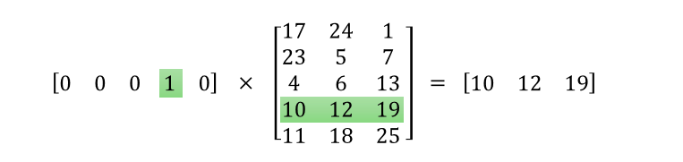
Since the input is a one-hot vector, the hidden activation is just a lookup operation. That is, hidden activation just looks up the row corresponding to the word ID in
Winput-hidden and passes it on to the output layer. As an illustration,
 Output Layer:
Target word - darkest
[0,0,0,1,0,0,0,0]
Output Layer:
Target word - darkest
[0,0,0,1,0,0,0,0]
Since the output layer is a
softmax layer, it produces a probability distribution across the words. Thus, the categorical logloss is calculated (and since this is a softmax, the error is just the difference between the target vector and the output vector). This error is then back propagated to the hidden layer.
As you might have noticed, this procedure gives us two trained parameters. The
Winput-hidden and
Whidden-output. Usually,
Whidden-output is discarded.
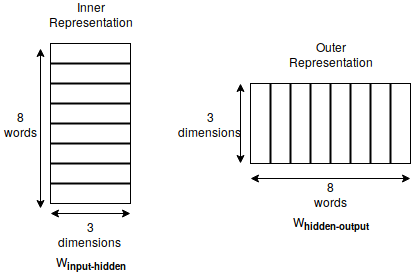
In the Mikolov's equation we saw above,
Vw is the
inner representation of the word i.e from
Winput-hidden and
VIw is the
outer representation of the word i.e from
Whidden-output.
Inner representation is nothing but the representation of the word when it is the current word and
outer representation is when the word occurs in the window of another word.
After the training process, the
Winput-hidden is just a lookup table, given the index, it returns the 3 bit
inner representation of the word. Similarly,
Whidden-output is a lookup table for the
outer representation of the word.
 Why does this work?
This method accomplishes dual task of reducing the dimensionality and adding semantic meaning to the word.
How?
Let us take 2 pairs of words.
('Computers', 'ML') and
('NFL', 'Kobe'). If we look at the above pairs, we can see that
'Computers' and
'ML' occur in the same context in the corpus. Hence, the representations of the words
'Computers' and
'ML' will be very close to each other (cosine similarity). Whereas, there is no way
'NFL' would be a part of a discussion about
'ML' (Although there is a Kobe challenge on Kaggle, which we are assuming is absent from the corpus) and hence the similarity between them will be very low. Since the context will be similar to
'Computer' and
'ML' and
'NFL' and
'Kobe', the neural net is forced to learn similar representations for each of these pairs.
This also handles stemming on a certain level, as
'Computers' and
'Computer' occur in the same context and can be interchanged. This also has the ability to handle acronyms. Since
'ML' and
'Machine' and
'Learning' occur in the same contexts, all 3 words will have similar representations.
One important thing to note is that Word2Vec does
not consider the positional variable of the context words i.e whether the word
'Learning' comes before
'Machine' or after is immaterial to the model. It does not learn a different vector for
'Learning' when it occurs before
'Machine' or after.
Here are some of the resources where you can find the detailed mathematical derivation for Word2Vec:
http://www.1-4-5.net/~dmm/ml/how_does_word2vec_work.pdf
http://www-personal.umich.edu/~ronxin/pdf/w2vexp.pdf
https://cs224d.stanford.edu/lectures/CS224d-Lecture2.pdf
01 Mar 2017
One of the most important aspects of any Natural Language Processing is the representation of the words. This throws up a unique problem of how to represent words in vector form. Words are ambiguous and can have multiple, complex relationships with other words. Additionally, the number of words in the vocabulary of any given language is in hundreds of thousands of magnitude.
One of the earliest attempts at word representation was made by WordNet, where each word was represented discretely and the relationships were established between words through hypernyms, synonyms etc. One of the main disadvantages of this setup was the amount of human intervention required to keep this corpus up-to-date. For a community that thrives on automation, this was just unacceptable. Additionally, this building of corpus was specific to a language. Building the corpus for any other language would require as much, if not more, effort and human intervention. Hence, this was not scalable.
Another discrete representation is one-hot representation (i.e creation of dummy variables). This is just a vector of size equal to the vocabulary size and each word is assigned an index. The one-hot vector of a word will be a vector filled with 0s with it's index bit set to 1. This representation also suffers from the same drawbacks as mentioned above. The vocabulary size of Google's corpus is about 13M. Hence each word would be required to be represented by a sparse vector of dimension 13M.
Another disadvantage of a one-hot representation is the underlying assumption that each word in the vocabulary is independent of each other, which is not the case. Since each word is represented by an arbitrary index, we cannot establish any implicit relationships between words.
In order to capture the semantics of any word and it's relationship to any other word, we need to look at the context in which the word appears. According to Richard Socher,
"You shall know a word by the company it keeps"
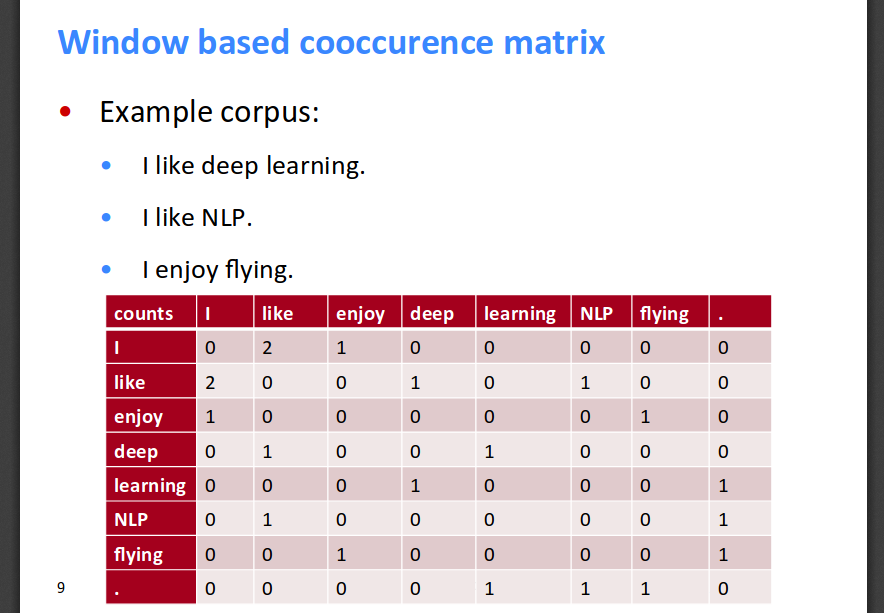
This gives us the idea that the representation of any word should be some function of the words surrounding the current word. One of the most intuitive ways of doing this is to use a co-occurrence matrix. This matrix just counts the number of times the current word is surrounded by another word.
There are two ways of taking the neighbours into account. One is to consider the document level frequency, where word frequencies are captured across documents. Second is to localize the context into neighbouring words (called windows). It is proven that the window based approach is better as it is capable of capturing both syntactic (Part-of-Speech) and semantic information.
The following is an example from Socher's slides, which better illustrates the co-occurrence matrix (for a window of size 1):

One of the drawbacks of using co-occurrence matrix is that some words like '
is', '
the', '
at' etc, which have a high frequency of occurrence in a corpus can skew the importance of features towards themselves. Easiest way of overcoming this is to remove the stop-words and cap the maximum frequency of occurrence of any word.
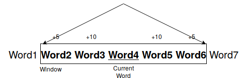
Another improvement to the window method is to use a ramped window method where more importance is given to the words immediately next to the current word, than words which are much further away.
Using this method, we can capture the semantics of the word up to some extent. But this method does not solve the problem of huge dimensionality of the word vector. It still remains the size of the vocabulary.
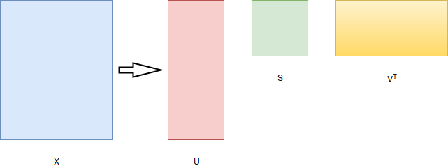
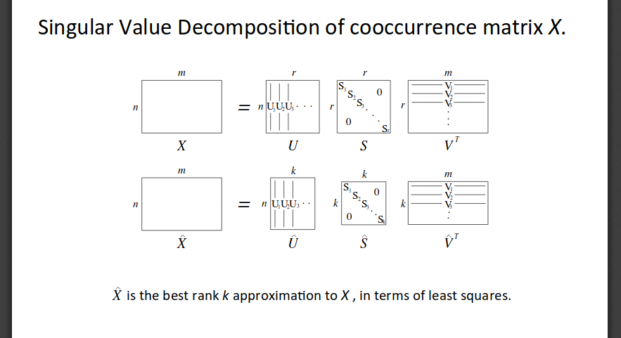
In order to reduce the dimension of the vector, we can leverage the age old linear algebraic method of Singular Value Decomposition (SVD).
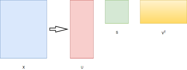
From Socher's slides,
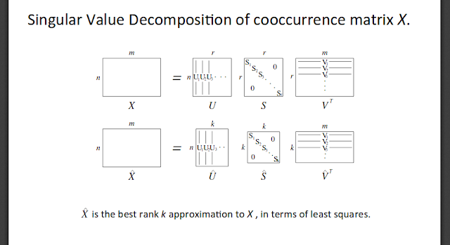
Here, \( S1, S2,...,Sn \) are arranged according to the importance of the dimensions.
Although SVD is a simple way of reducing the dimensionality of the vector, it is computationally very expensive and it is difficult to add new words to the vocabulary (Since the matrix has to be decomposed every time the input matrix changes).
Hence, we use Word2Vec, a pseudo-neural approach of solving dimension reduction while preserving the semantic information of a co-occurrence matrix. There will be a separate post exploring Word2Vec in detail.
For more reference, refer Socher's slides at:
Stanford: Word Vectors