Interpreting Machine Learning Models - Introduction

One of the main impediments to the wide adoption of machine learning, especially deep learning, in critical (and commercial) applications is the apparent lack of trust accorded to these machine learning applications. This distrust mainly stems from the inability to reason about the outputs spit out by these models. This phenomenon is not just relegated to those who are outside the machine learning domain either. Even seasoned machine learning practitioners are flummoxed by the apparent failings of machine learning models. In fact, I would go so far as to say that longer you tinker around machine learning, more skeptical you become of its’ abilities.

Extensive research and development has been done in machine learning domain in the past decade and almost all of it has concentrated on achieving that elusive 100% accuracy (or whatever other metrics are used) and most of it were still in the research labs, with nary a thought given to the issue of how exactly this would be applied in the real world. With billions of dollars being poured into this domain and after years in research labs, it was time to bring this technology out in the open for commercial use. This was when the true drawback of integrating machine learning into our everyday lives became apparent. It is not so easy to trust a machine learning model.

If we delve deeper into why it is hard for us to trust a machine learning model, it helps to look into how we handle decisions taken by others that affect us. We, as humans, tend to give more importance to how a decision was arrived at rather than the decision itself. Taking an advisor-investor relationship as an example, if the advisor recommends a particular stock to the investor, he needs to explain why he came to that decision. Even if the investor is not as savvy as the advisor and might not grasp all the decision making factors of the advisor, he will be wary of investing without any type of explanation. And if the advisor insists on not providing any explanation, it would erode the trust between them. Similarly, all the machine learning models are “decision-making” models and we need to be able to “see” how a model arrived at an output even if it doesn’t make complete sense to us.

Another reason why we have so little trust in machine learning models is because of the paucity of understanding in how exactly these models interpret the real world. Even if we have a state-of-the-art model that achieves 99.9% accuracy, we do not know why it fails in the other 0.1%. If we knew, we would fix it and achieve 100%. We cannot trust any machine learning output completely because we do not know when it is going to fail. This drawback became apparent with the introduction of adversarial networks and their runaway success in breaking almost all the state-of-the-art models at the time. Turns out, we do not exactly know how an object detector model exactly detects an object even though we know enough to push it to 99.9%.

Now that we are faced with the reality of deploying these models in the real world and asking people to use them and consequently trust them (sometimes with our lives, as is the case in self driving automobiles), we have to invest more in interpreting the outputs of these models. We are seeing more and more research being done on interpretability of machine learning models in recent times. This is not cure-all for widespread adoption of machine learning, but it is definitely a good starting point.

The purpose of this blog series is to explore some of the ways we can achieve machine learning interpretability and keep this in mind before developing any new machine learning applications.

Links to the blog series:

1. Part 1: Evaluation and Consequences
2. Part 2: Interpretable Machine Learning Models

Citations:

• Molnar, Christoph. “Interpretable machine learning. A Guide for Making Black Box Models Explainable”, 2019. https://christophm.github.io/interpretable-ml-book/.
• Explainable AI for Science and Medicine by Microsoft
• Software for Explainable AI

Google Search by Voice - Case Study Summary

This blog post is a summary of the case study made by Google when it first launched it’s voice services. For any company/person trying to undertake this endeavor of building a voice product, this early stage case study is a huge knowledge bank. For one, it is always better to learn from someone else’s mistake rather than our own and two, majority of the underlying architecture of Google’s voice platform has remained the same over the years. Going through this case study gives us an important insight into how Google does voice.

The original case study file can be found here

If you are new to Speech and Speech Recognition, I would recommend you to start here: Introduction to Automatic Speech Recognition

GOOG-411

GOOG-411 was a domain specific Automatic Speech Recognizer(ASR)/Language Model(LM) for telephone directory listings.

GOOG411: Calls recorded...  Google! What city and state?
Caller : Palo Alto, California
GOOG411: What listing?
Caller : Patxis Chicago Pizza
GOOG411: Patxis Chicago Pizza, on Emerson Street. I’ll connect you...

Instead of 2 separate queries, in 2008 a new version of GOOG-411 was released which could take both entities as input in a single sentence.

GOOG411: Google! Say the business, and the city and state.
Caller : Patxis Chicago Pizza in Palo Alto.
GOOG411: Patxis Chicago Pizza, on Emerson Street. I’ll connect you...

In November 2008, Voice Search was first deployed for Google app users in iPhone.

Challenges in handling search compared to domain specific applications:

• Complex grammar support is required
• Need to support huge vocabulary.

Metrics

1. WER:

   \[WER = \frac{\text{No of substitutions} + \text{insertions} + \text{deletions}}{\text{Total number of words}}\]

2. Semantic Quality (WebScore): WER is not an accurate depiction of usability of an ASR system. For eg, even if we error on some filler words like “a”, “an”, “the” etc, we can still reliably do accurate entity extraction. Hence, we should optimize on this metric rather than on WER.

   Logic is simple. Take the output from ASR. Run it through the search engine and get the results. Take the correct transcription. Run it through the search engine and get the results. The amount of overlap between these two results shows how good/usable the ASR is.

   Google’s WebScore is calculated as follows:

   \[WebScore = \frac{\text{Number of correct web results}}{\text{Total number of spoken queries}}\]

3. Perplexity: This is a measure of the how confident the system is about a result. Lower the perplexity, better the system is.

4. Out of Vocabulary (OOV) Rate: The out-of-vocabulary rate tracks the percentage of words spoken by the user that are not modeled by the language model. It is important to keep this number as low as possible.

5. Latency: Reaction time of the system. Total time taken from the user speaking to producing relevant results to him. Lower the latency, better the UX.

Acoustic Modeling

The details of these systems are extensive, but improving models typically includes getting training data that’s strongly matched to the particular task and growing the numbers of parameters in the models to better characterize the observed distributions. Larger amounts of training data allow more parameters to be reliably estimated.

Two levels of bootstrapping required:

1. Once a starting corpus is collected, there are bootstrap training techniques to grow acoustic models starting with very simple models (i.e., single-Gaussian context-independent systems.
2. In order to collect ‘real data’ matched to users actually interacting with the system, we need an initial system with acoustic and language models.

For Google Search by Voice, GOOG-411 acoustic models were used together with a language model estimated from web query data.

Large amounts of data starts to come in once the system goes live and we need to leverage this somehow

1. Supervised Labeling where we pay human transcribers to write what is heard in the utterances.
2. Unsupervised Labeling where we rely on confidence metrics from the recognizer and other parts of the system together with the actions of the user to select utterances which we think the recognition result was likely to be correct.

Model architecture:

39-dimensional PLP-cepstral coefficients together with online cepstral normalization, LDA (stacking 9 frames) and STC. The acoustic models are triphone systems grown from deci-sion trees, and use GMMs with variable numbers of Gaussians per acoustic state, optimizing ML, MMI, and ‘boosted‘-MMI objective functions in training.

Observed effects:

• The first is the expected result that adding more data helps, especially if we can keep increasing the model size.
• It is also seen that most of the wins come from optimizations close to the final training stages. Particularly, once they moved to ‘elastic models’ that use different numbers of Gaussians for different acoustic states (based on the number of frames of data aligned with the state), they saw very little change with wide ranging differences indecision tree structure.
• Similarly, with reasonably well-defined final models, optimizations of LDA and CI modeling stages have not led to obvious wins with the final models.
• Finally, their systems currently see a mix of 16 kHz and 8 kHz data. While they’ve seen improvements from modeling 16 kHz data directly (compared to modeling only the lower frequencies of the same 16kHz data), so far they do better on both 16 kHz and 8 kHz tests by mixing all of their data and only using spectra from the first 4 kHz of the 16 kHz data. They expect this result to change as more traffic migrates to 16 kHz.

Next challenge: Scaling

Some observations:

• The optimal model size is linked to the objective function: the best MMI models may come from ML models that are smaller than the best ML models
• MMI objective functions may scale well with increasing unsupervised data
• Speaker clustering techniques may show promise for exploiting increasing amounts of data
• Combinations of multi-core decoding, optimizations of Gaussian selection in acoustic scoring, and multi-pass recognition provide suitable paths for increasing the scale of acoustic models in realtime systems.

Text Normalisation

Google uses written queries to google.com in order to bootstrap their language model (LM) for Google search by Voice. The large pool of available queries allowed them to create rich models. However, they had to transform written form into spoken form prior to training. Analyzing the top million vocabulary items before text normalization they saw approximately 20% URLs and 20+% numeric items in the query stream.

Google uses transducers (FSTs) for text normalisation. See the Finite State Transducer section in blog post for an introduction to what transducers are.

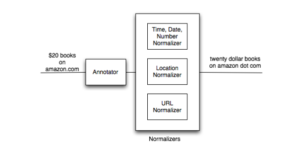
In the annotator phase, they classify parts (sub strings) of queries into a set of known categories (e.g time, date, URL, location). Once the query is annotated, each category has a corresponding text normalization transducer \(N_{cat}(spoken)\) that is used to normalize the sub-string. Depending on the category they either use rule based approaches or a statistical approach to construct the text normalization transducer. They used rule based transducer for normalizing numbers and dates while a statistical transducer was used to normalize URLs.

Large scale Language Modeling (LM)

Ideally one would build a language model on spoken queries. As mentioned above, to bootstrap they started from written queries (typed) to google.com. After text normalization they selected the top 1 million words. This resulted in an out-of-vocabulary (OOV) rate of 0.57%. Language Model requires aggressive pruning (to about 0.1% of its unpruned size). The perplexity hit taken by pruning the LM is significant - 50% relative. Similarly, the 3-gram hit ratio is halved.

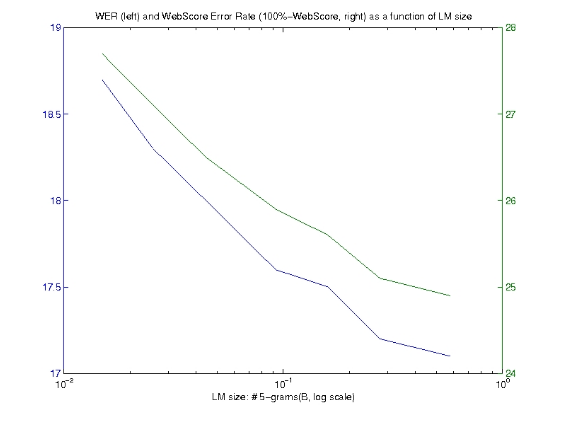
The question they wanted to ask was, how does the size of the language model affect the performance of the system. Are these huge numbers of n-grams that we derive from the query data important?

Answer was, as the size of the language model increased, a substantial reduction in both the Word Error Rate (WER) and associated WebScore was observed.

Locale Matters (A LOT):

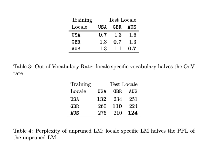
They built locale specific English language models using training data from prior to September 2008 across 3 English locales: USA, Britain, and Australia. The test data consisted of 10k queries for each locale sampled randomly from Sept-Dec 2008. The dependence on locale was surprisingly strong: using an LM on out-of-locale test data doubled the OOV rate and perplexity.

They also built a combined model by pooling all data. Combining the data negatively impacts all locales. The farther the locale from USA (as seen on the first line, GBR is closer to USA than AUS), the more negative the impact of clumping all the data together, relative to using only the data from that given locale.

In summary, locale-matched training data resulted in higher quality language models for the three English locales tested.

User Interface

“Multi Modal”: Meaning different forms of interaction. For eg, telephone is a single modal UI since the input and output is voice. Google Search by Voice is multi modal since input is voice and output is visual/text and similarly, Maps is multi modal since input is voice and output is graphics.

Advantages of multi modal outputs:

1. Spoken input vs output

   There are two different scenarios in using Search by Voice. If we are searching for a specific item, single modal response is a good UX. If we are searching using a broader term for search or the user wants to explore/browse further, single modal results in a bad UX. The following illustrates this:

   Good UX:

    GOOG411: Calls recorded... Google! Say the business and the city and state.
    Caller : Patxi’s Chicago Pizza in Palo Alto.
    GOOG411: Patxi’s Chicago Pizza, on Emerson Street. I’ll connect you...
   

   Bad UX:

    GOOG411: Calls recorded... Google! Say the business and the city and state.
    Caller : Pizza in Palo Alto.
    GOOG411: Pizza in Palo Alto... Top eight results:
             Number 1: Patxi’s Chicago Pizza, on Emerson StreetTo select number one, press 1 or say ”number one”.
             Number 2: Pizza My Heart, on University Avenue.
             Number 3: Pizza Chicago, on El Camino Real.[...]
             Number 8: Spot a Pizza Place: Alma-Hamilton, on Hamilton Avenue
   

2. User control and flexibility:

   Unlike with voice-only applications, which prompt users for what to say and how to say it, mobile voice search is completely user-initiated. That is, the user decides what to say, when to say it and how to say it. There’s no penalty for starting over or modifying a search. There’s no chance of an accidental “hang-up” due to subsequent recognition errors or timeouts. In other words, it’s a far cry from the predetermined dialog flows of voice-only applications.

The case study explored further on UI/UX observations regarding visual interfaces, including how and where the button should be placed, how to show the ASR alternatives, intent based navigation to apps (Drive to vs Navigate to) etc

Ubuntu and Debian Package Management Tutorial

Package management is one of the components that contribute to the steep learning curve of using a linux system for a majority of first time linux users. Coming from the GUI environment of Windows or MacOS where installing/removing applications consist of clicking on Next -> Next -> I Agree -> Install/Uninstall, the terminal based package managers might be intimidating. And this issue is not constrained to first time users either. Even though I have used a linux system as my primary OS for several years now, I end up googling the errors and copy-pasting the answers from SO without the slightest idea of what I am doing most of the times. Hence, I am writing this blog post to be a glossary of the commands that we can use to fix our own package errors or to know what each command is doing even if we end up copy-pasting from the internet to fix our problems.

RHEL-based distributions:

• Packaging format: RPM
• Tools: rpm, yum

Debian and Ubuntu based distributions:

• Packaging format: .deb
• Tools: apt, apt-get, dpkg

In this blog post, I will be covering the Debian/Ubuntu based distributions, since well, I am a Ubuntu user.

Debian/Ubuntu Package Management Tools

• apt-get:

  apt-get is used to interface with remote repositories. Main difference with apt is that apt pulls from the remote repository into a local cache and then uses this copy in the cache. apt-get uses the same methodology but refreshes the cache every time.

• apt-cache:

  Like discussed earlier, this is the local cache that apt uses.

• aptitude:

  Has both capabilities of the above tools. Can be dropped in place of both apt-get and apt-cache.

• dpkg:

  The above tools are used to manage and pull packages from remote repositories. dpkg operates on the actual .deb files. It cannot resolve dependencies like apt-*.

• tasksel:

  This is used for grouping of similarly related packages. For eg, if you want a MEAN stack setup, you can use tasksel to install all required packages instead of installing each of them individually.

Commands

1. sudo apt-get update

   Updating the local cache with the latest info about the remote repositories.

2. sudo apt-get upgrade

   Upgrade any component that do not require you to remove any other packages.

3. sudo apt-get dist-upgrade

   Upgrade components when you are OK with removing/swapping other packages.

4. apt-cache search _package_

   Search for package in the repositories. You will have to run sudo apt-get update before doing this.

5. sudo apt-get install _package_

6. sudo apt-get install _package1_ _package2_

7. sudo apt-get install _package=version_

   Install a specific version of the package.

8. sudo dpkg-reconfigure _package_

   Reconfigure package. Most of the packages, after you install them, they go through a configuration script that configures your system to use that particular package. Sometimes this include user prompts as well. If you want to do this configuration yourself after installation or rerun the configuration, use this command.

9. apt-get install -s _package_

   Dry-run installation. Using this command you can see all the changes that installing package might do to your system without actually doing those changes. One important note is that this command does not require sudo and hence can be used in systems where you do not have root privileges.

10. sudo dpkg --install _debfile.deb_

    Install directly from the debfile.deb file. Note that this DOES NOT resolve dependencies.

11. sudo apt-get install -f

    This command is used to fix dependency issues. While installing a package, if there are unmet dependencies, the installation will fail. If you’ve noticed, apt-* commands resolve these dependencies automatically. Whereas using dpkg to install .deb files directly does not resolve dependencies. Hence, run this command in those scenarios.

12. sudo apt-get remove _package_

    Remove the package without removing the configuration files. If you accidentally remove a package or install the same package after some time, you will need to save the configuration you did for your first installation.

13. sudo apt-get purge _package_

    Remove the package and all it’s configuration files.

14. sudo apt-get autoremove

    Remove any packages that were installed as dependencies and are no longer required. Use --purge to remove the configuration files of these packages.

15. sudo apt-get autoclean

    Remove out-of-date packages in your system that are no longer maintained in the remote repository.

16. apt-cache show _package_

    Show information about package.

17. dpkg --info _debfile.deb_

    Show information about the debfile.deb file.

18. apt-cache depends _package_

    Show dependencies of the package.

19. apt-cache rdepends _package_

    Show packages that are dependent on this package (reverse dependency)

20. apt-cache policy _package_

    If there are multiple versions of package installed, this command shows all the versions and the version being used as default.

21. dpkg -l

    Shows a list of every installed/partially-installed packages in the system. Each package is preceded by a series of characters.

    First character:

    - _u_: unknown
    - _i_: installed
    - _r_: removed
    - _p_: purged
    - _h_: version is held
    

    Second character:

    - _n_: not installed
    - _i_: installed
    - _c_: configuration files are present, but the application is uninstalled
    - _u_: unpacked. The files are unpacked, but not configured yet
    - _f_: package is half installed, meaning that there was a failure part way through an installation that halted the operation
    - _w_: package is waiting for a trigger from a separate package
    - _p_: package has been triggered by another package
    

    Third character:

    - _r_: re-installation is required. Package is broken.
    

22. dpkg -l _regex_

    Search for all packages matching the regex.

23. dpkg -L _package_

    List all files controlled by this package.

24. dpkg -S _/path/to/file_

    This is the inverse of -L, which gives a list of all files controlled by a package. -S prints the package that is controlling this file.

25. dpkg --get-selections > ~/packagelist.txt

    Export the list of installed packages to ~/packagelist.txt file which can be used to restore in a new system. This is analogous to requirements.txt file in python.

26. sudo add-apt-repository _ppa:owner_name/ppa_name_

    This is used to add a PPA (Personal Package Archives). When you cannot find the required package in the default set of repositories and is available in another repository, we can add that PPA and install packages from there. This is specific to Ubuntu systems as of now. Before installing packages from the newly added repository, update the local cache with sudo apt-get update. Usually PPAs have a smaller scope than a repository.

27. Adding a new repository:
    • Edit the /etc/apt/sources.list file

    • Create a new /etc/apt/sources.list.d/new_repo.list file (Must end with .list)

      Inside the file, add the new repository with the following format. deb_or_deb-src url_of_repo release_code_name_or_suite component_names

    • deb or deb-src: This identifies the type of repository. It can be either deb (for conventional repositories) or deb-src (for source repositories)
    • url: URL of the repository.
    • release_code_name or suite: Code name of your distribution’s release
    • component_names: Labels for the source.

28. Exporting a package list:

    If you want to setup a new system with all the packages from the old system, you first have to export the package details from the old system and install it in the new system.

    • dpkg --get-selections > ~/packagelist.txt: Export all package names
    • mkdir ~/sources
    • cp -R /etc/apt/sources.list* ~/sources: Backup your sources list.
    • apt-key exportall > ~/trusted_keys.txt: Backup your trusted keys
29. Importing a package list:
    • sudo apt-key add ~/trusted_keys.txt
    • sudo cp -R ~sources/* /etc/apt/
    • sudo dpkg --clear-selections: Clear all non essential packages from the system for a clean slate.
    • sudo apt-get update
    • sudo apt-get install dselect: Install dselect tool
    • sudo dselect update
    • sudo dpkg --set-selections < packagelist.txt: Import from the package list.
    • sudo apt-get dselect-upgrade

Decoding (ASR Part 4)

Link to the start of ASR series: Automatic Speech Recognition (ASR Part 0)

Now that we have explored Acoustic Modeling and Language Modeling, the next logical question is, how do we put these things together? Running both AM and LM and combining the results into a list of hypothesis is called as the Decoding Process and this is harder than it looks mainly because of latency and speed concerns which have an adverse effect on RTF.

Decoding Speed

Decoding speed is usually measured with respect to a real-time factor (RTF). A RTF of 1.0 means that the system processes the data in real-time, takes ten seconds to process ten seconds of audio. Factors above 1.0 indicate that the system needs more time to process the data (Used in meeting transcriptions). When the RTF is below 1.0, the system processes the data more quickly than it arrives. For instance, when performing a remote voice query on the phone, network congestion can cause gaps and delays in receiving the audio at the server. If the ASR system can process data in faster than real-time, it can catch up after the data arrives, hiding the latency behind the speed of the recognition system.

The solution to a majority of latency issues in computer engineering lies in data structures. ASR decoding is no different. In order to make decoding easier, we represent both the AM and the LM as Weighted Finite State Transducers (WFSTs). This brings with it all the capabilities of WFST operations to AM and LM in order to combine them.

Before we dive into WFST, there are other data structures that we need to be introduced to.

Finite State Acceptor (FSA)

Finite representation of a possibly infinite set of strings. It is a Finite State Machine (FSM) where there are states (INITIAL and FINAL). Transition from one state to the other is by consuming a letter (let us call this input).

Weighted Finite State Acceptor (WFSA)

WFSA is similar to FSA except that there is a cost associated with each state change. Cost is multiplied along one path and added across paths. Therefore, even though there are multiple ways of going from the initial state to the final state, we take the path with min cost.

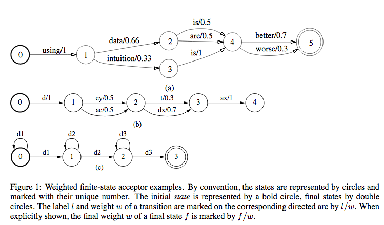
In the above figure, we can see 3 types of applications of WFSAs in ASRs.

1. Figure 1(a): Finite state language model
2. Figure 1(b): Possible pronunciations of the word \(\text{data}\) used in the language model
3. Figure 1(c): 3-distribution-HMM structure for one phone, with the labels along a complete path specifying legal strings of acoustic distributions for that phone.

Finite State Transducer (FST)

FST is similar to FSA except that for each arc, we have both input and output symbols. For the corresponding state transition, we consume the input symbol and emit the output symbol.

Weighted Finite State Transducer (WFST)

WFST is similar to FST except that there is a cost associated with each state change. All the operations on cost that we perform on WFSA are applicable here too.

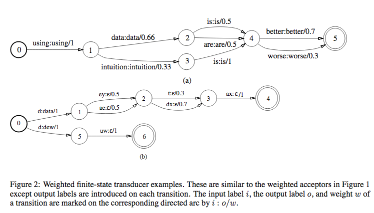
The figure above is same as the WFSA but with input:output on each state instead of just input. \(\epsilon\) is a null symbol.

Now that we know what FSA, WFSA, FST and WFST are, why do we choose WFST over other data structures to represent models in our ASR? WFST (which is a transducer) can represent a relationship between two levels of representation, for eg, between phones and words (like figure 2(b)) or between HMMs and context-independent phones.

• WFST Union: Combine transducers in parallel
• WFST Concatenation: Combine transducers in series
• Kleene Closure: Combine transducers with arbitrary repetition (With * or +)

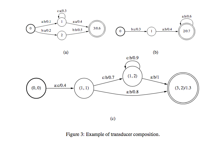
Operations on WFSTs

• Composition

If there are two transducers \(T_{1}\) and \(T_{2}\) and their composition is \(T\), we represent \(T=T_{1} \circ T_{2}\). If \(T_{1}\) takes \(u\) as input and gives \(v\) as output and \(T_{2}\) takes \(v\) as input and gives \(w\) was output, then \(T\) takes \(u\) as input and gives \(w\) as output. Weights in \(T\) is computed from the weights in \(T_{1}\) and \(T_{2}\) (maybe product (in case of prob) or sum (in case of log)).

• Determinization

In this, WFSTs should satisfy the following conditions:

• From any state, for a given input, there should be only one transition
• No \(\epsilon\) symbols in input

The above conditions make it easier to compute determinization since from each state, we have only one transition for one input symbol.

• Minimization

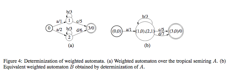
This is to simplify the structure of the WFST.

WFST in Speech

WFSTs are used in the Decoding Stage. (WFST Speech Decoders). WFST is a way of representing HMMs, statistical language models, lexicons etc.

There are four principal models for speech recognition:

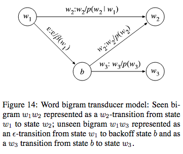
1. Word Level Grammar\((G)\): In \(G\), every word is considered to be a state. If we take a bigram model, there is a transition from \(w_{1}\) to \(w_{2}\) for every bigram \(w_{1}w_{2}\) in the corpus. The weight for this transition will be \(-log(p(w_{2}|w_{1}))\). We use \(\epsilon\) to represent unseen bigrams, for eg, \(w_{1}w_{3}\)

2. Pronunciation Lexicon\((L)\): This transducer is non determinizable due to the following reasons:
   • Homophones: Different words are pronounced the same, and hence will have the same sequence of phones.
   • First word of the output string might not be known before the entire phone string is scanned: For eg, if we take the sequence of phones (corresponding to the word \(\text{"carla"}\)), we cannot say that the word is \(\text{"car"}\) before consuming the entire sequence.

   In order to overcome this, we use a special symbol #_{0} to mark the end of phonetic transcription of a word. In order to distinguish between homophones, we use other symbols such as #_{1}...#_{k-1}. For eg, \(\text{"red"}\) is r eh d #_{0} and \(\text{"read"}\) is r eh d #_{1}.

3. Context Dependency Transducer\((C)\): We denote context dependent units as phone/leftcontext_rightcontext.
4. HMM Transducer\((H)\)

Consider the WFSTs in Figure 2. Figure 2(a) is the grammar \(G\) and in Figure 2(b) we have pronunciation lexicons \(L\). If we do a composition of these two transducers, we get a new transducer that takes phones as input and gives words as output (These words are restricted to the grammar \(G\) since \(G\) can’t accept any other words). So, we get \(L \circ G\).

The above composition is just a context independent substitution (Monophone model).

In order to get context dependent substitution, we again use composition on top of context independent substitution (called Triphone model).

Let us take the word \(\text{"cat"}\) as an example. The sequence of phonemes for this word is \(k\), \(\text{ae}\), \(t\). Let us assume that the notation \(\text{ae/k_t}\) represents a triphone model for \(\text{ae}\) with left context \(k\) and right context \(t\).

We have the following state transitions for the triphone model.

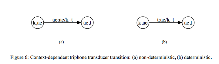
The above transducer that maps context independent phones to context dependent phones is denoted by \(C\). Hence, we get \(C \circ (L \circ G)\).

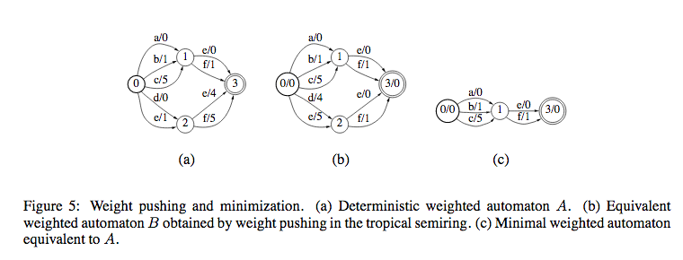
After this, we perform Determinization and Minimization on this.

Adding HMM to model the input distribution, WFST for speech recognition can be represented as a transducer which maps from distributions to words strings restricted to G.

References

• Dixon Tutorial
• Speech Recognition with WFSTs

Language Modeling (ASR Part 3)

Link to the start of ASR series: Automatic Speech Recognition (ASR Part 0)

Language Modeling is the technique of modeling a system that assigns probabilities to a sequence of words. Language Models (LMs) model valid sequences of words in a language that are sematically and syntactically correct and is used to differentiate between valid sentences in a language and random sequences of words. This is achieved by modeling the probability of a word occurring in a given sentence given it’s predecessors.

Given that we are building an ASR system, how is LM relevant in this case? An AM gives us the probable word given it’s acoustic representation (MFCC). Given a series of continuous acoustic vectors, AM spits out a distribution over all the words in the dictionary at each time step. Just taking the maximum word at each time step will not yield correct results for the basic fact that each word is dependent on the surrounding words. For example, the acoustic representation of the words \(\text{"ball"}\) and \(\text{"wall"}\) would be similar to each other and the AM will assign high scores to these words. But choosing the correct word among these is subject to the context of the sentence. If the surrounding words are related to sports (let’s say) then we should choose \(\text{"ball"}\) even if it has a lower AM score. This decision of choosing the correct word given it’s context is done by LM.

There are different LMs employed in active use today. Some of the bleeding edge LMs are deep neural networks (Deep Bi-LSTM networks specifically).

We will be exploring one of the widely tested LMs in this blog post.

N-Gram Language Model

For a bigram,

For an N-gram,

In this case, for unseen words, we get 0 probability. Hence we need to do some smoothing. Similar to Add One Smoothing (also called as Laplace Smoothing), we have Witten Bell Smoothing. Here, while calculating the probabilities of seen N-grams, we need to keep aside some probability for unseen stuff.

For eg, in case of unigrams, we usually do,

For an unseen word, it will be 0. So instead of the above we do this,

\(P(word) = \frac{c(word)}{c(\text{all_words})+V}\), where \(V\) is the vocabulary size.

Similarly, for N-gram, we do,

where, \(V(w_{1}w_{2}...w_{k-1})\) is the number of unique words that follows these words.

Back Off Strategy

Let us take a look at this scenario. We have a 4-gram \(\text{"tiger killed wild boar"}\) and we need to calculate,

Assume that this 4-gram does not occur in the training corpus, i.e

Then, we split the above into,

If this trigram is also not present in the corpus, i.e

Then we again split into,

and so on until we get a count that is not 0.

Therefore, we get,

This technique is called Backoff strategy.

Language Model Evaluation

Likelihood

For a bigram model, for sentences in a test set, probability is computed as,

where \(<s>\) is the sentence-start token and \(</s>\) is the sentence-end token.

If we have 2 models A and B, whichever gives the higher probability values to these words in the test set is a better model.

Log Likelihood

In the above equation, since we are multiplying numbers less than one, the number becomes too small too quickly. Hence, we take log on both sides.

Entropy

If we multiply the above the equation by \(-\frac{1}{n}\), we get entropy.

Perplexity

Perplexity is the average reciprocal of the word probability. So, if words on average are assigned probability 1/100 then the perplexity would be 100.

Perplexity is just the anti-logarithm (exponential) of the entropy.

To explain perplexity further,

Removing \(log\),

Hence,

To summarize LM evaluations,

HIGH likelihood ↔ LOW entropy ↔ LOW perplexity ↔ GOOD model

LOW likelihood ↔ HIGH entropy ↔ HIGH perplexity ↔ BAD model

Modern Language Models

• Universal Language Model by fast.ai
• Universal Sentence Encoder by Google
• Deep Averaging Networks
• Transformers
• BERT
• ELMo
• ELMo Blog