05 Dec 2018
Link to the start of ASR series: Automatic Speech Recognition (ASR Part 0)
This blog post explores the acoustic modeling component of ASR systems.
Phonetics
Phonetics is the part of linguistics that focuses on the study of the sounds produced by human speech. It encompasses their production (through the human vocal apparatus), their acoustic properties, and perception. The atomic unit of speech sound is called a phoneme. Words are comprised of one or more phonemes in sequence. The acoustic realization of a phoneme is called a phone.
There are three basic branches of phonetics, all of which are relevant to automatic speech recognition.
- Articulatory phonetics: Focuses on the production of speech sounds via the vocal tract, and various articulators.
- Acoustic phonetics: Focuses on the transmission of speech sounds from a speaker to a listener.
- Auditory phonetics: Focuses on the reception and perception of speech sounds by the listener.
Syllable
A syllable is a sequence of speech sounds, composed of a nucleus phone and optional initial and final phones. The nucleus is typically a vowel or syllabic consonant, and is the voiced sound that can be shouted or sung.
As an example, the English word \(\text{"bottle"}\) contains two syllables. The first syllable has three phones, which are \(b aa t\) in the Arpabet phonetic transcription code. The \(aa\) is the nucleus, the \(b\) is a voiced consonant initial phone, and the \(t\) is an unvoiced consonant final phone. The second syllable consists only of the syllabic cosonant \(l\).
Acoustic Modeling
Acoustic Model is a classifier which predicts the phonemes given audio input. Acoustic Model is a hybrid model which uses deep neural networks for frame level predictions and HMM to transform these into sequential predictions.
The three fundamental problems solved by HMMs:
- Evaluation Problem: Given a model and an observation sequence, what is the probability that these observations were generated by the model? (Forward Algorithm)
- Decoding Problem: Given a model and an observation sequence, what is the most likely sequence of states through the model that can explain the observations? (Viterbi Algorithm)
- Training Problem: Given a model and an observation sequence (or a set of observation sequences) how can we adjust the model parameters? (Baum Welch Algorithm)
Mathematical foundation to HMMs can be found in this post
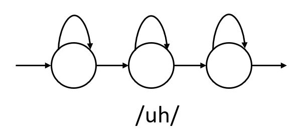
Each phoneme will be modeled using a 3 state HMM (beginning, middle and end)
Word HMMs can be formed by concatenating its constituent phoneme HMMs. For example, the HMM word \(\text{"cup"}\) can be formed by concatenating the HMMs for its three phonemes.
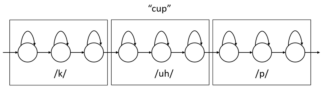
Therefore for training an Acoustic Model we need a word and its “spelling” in phonemes.
In HMM, each state has distribution over the observables (transition probabilities i.e a probability distribution over all the observable states from each hidden state). This distribution is modeled using a Guassian Mixture Models (GMM). There will be a separate GMM for each hidden state.
\[p(x|s) = \sum_{m}^{}w_{m}N(x;\mu_{m},\sum_{m})\]
where \(N(x;\mu_{m},\sum_{m})\) is Guassian Distribution and \(w_{m}\) is a mixture weight and \(\sum_{m}^{}w_{m} = 1\).
Thus, each state of the model has its own GMM. The Baum-Welch training algorithm estimated all the transition probabilities as well as the means, variances, and mixture weights of all GMMs.
Modern speech recognition systems no longer model the observations using a collection of Gaussian mixture models but rather a single deep neural network that has output labels that represent the state labels of all HMMs states of all phonemes. For example, if there were 40 phonemes and each has a 3-state HMM, the neural network would have \(40 \times 3 = 120\) output labels. Such acoustic models are called “hybrid” systems or DNN-HMM systems to reflect the fact that the observation probability estimation (transition probability) formerly done by GMMs is now done by a DNN, but that the rest of the HMM framework, in particular the HMM state topologies and transition probabilities, are still used. In simpler words, given an input MFCC vector, DNN will tell you what state it is in and of what phoneme. For eg, it might say that it is in the starting state of the phoneme \(/uh/\). Now, transitioning from this state to other state is handled by HMM.
Context Dependent Phones
In the previous section, we did context independent phones. For eg, for \(\text{"cup"}\), each phone \(/k/\), \(/uh/\), \(/p/\) were independent. In context dependent, each phone will have a preceding phoneme and succeeding phoneme which will be modeled. For eg, for \(\text{"cup"}\), HMM will look like this.
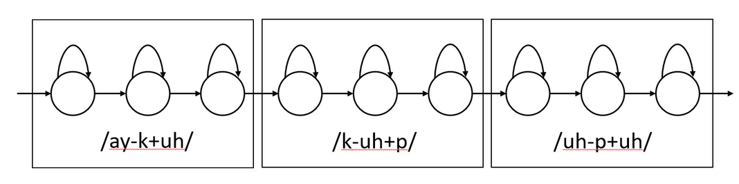
Because this choice of context-dependent phones models 3 consecutive phones, they are referred to as “triphones”. “quinphones” have a sequence of 5 consecutive phones.
In the previous example, we saw that since there were 40 phonemes and 3 states in each, we got 120 output labels. If we consider a triphone, number of phones will be \(40 \times 40 \times 40\) and 3 states each. Hence, we get 192,000 output labels.
This explosion of label space leads to 2 problems:
- Less data for training each triphone
- Some triphones will not occur in training but will occur in testing
Solution to this problem is clustering. Cluster groups of triphones which are similar to each other into groups called “senones”. Grouping a set of context-dependent triphone states into a collection of senones is performed using a decision-tree clustering process. A decision tree is constructed for every state of every context-independent phone.
Steps to cluster:
- Merge all triphones with a common center phone from a particular state together to form the root node. For example, state 2 of all triphones of the form /-p+/.
- Grow the decision tree by asking a series of linguistic binary questions about the left or right context of the triphones. For example, “Is the left context phone a back vowel?” or “Is the right context phone voiced?”. At each node, choose the question with results in the largest increase in likelihood of the training data.
- Continue to grow the tree until the desired number of nodes are obtained or the likelihood increase of a further split is below a threshold.
- The leaves of this tree define the senones for this context-dependent phone state.
Doing this, reduces 192,000 triphones to about 10,000 senones. As you might have guessed, now we will be doing classification for senones instead of phones/triphones. Therefore, there will be a GMM for each senone. In hybrid, since we are replacing the GMM with DNN, there will be \((\text{number_of_senones} \times 3)\) output labels.
Sequence Based Objective Functions
In frame-based cross entropy, any incorrect class is penalized equally, even if that incorrect class would never be proposed in decoding due to HMM state topology or the language model. With sequence training, the competitors to the correct class are determined by performing a decoding of the training data.
- Maximum Mutual Information (MMI)
- Minimum Phone Error (MPI)
- state-level Minimum Bayes Risk (sMBR)
Summary
So now we have a feed forward neural network that predicts which phoneme and which state. This is still frame independent i.e this is done for each frame. But in order to make it accurate, we append the previous frames and future frames to the current frame and give it as input.
Instead of this, we can as well train an RNN (with LSTM, GRU or a BiLSTM) which takes each frame in each time step and gives a prediction. But still, this is a frame independent procedure. (As an aside note, we need senone labels for each frame to train this network. That is generated by forced alignment. For forced alignment, we need an already trained speech recognizer to do the HMM decoding stage).
There is a disadvantage to this frame independent prediction. In cross entropy, we penalize all wrong classes equally. But for one target senone, there will be a set of commonly confused senones which have to be penalized more than others. This is where sequence objective functions come into picture instead of standard cross entropy.
04 Dec 2018
Link to the start of ASR series: Automatic Speech Recognition (ASR Part 0)
Input to the ASR system will be an audio file/stream that encodes the speech. How this speech is stored, transmitted and encoded is explored in this post.
How humans produce and perceive speech is vastly different from how we intuitively try to understand speech. Speech consists of multiple deterministic signals interspersed within indeterministic boundaries.
Human Ear
Human ear can perceive sounds with frequencies in the range \(20Hz\) to \(20kHz\). But this is not linear i.e we are more sensitive to lower frequencies than higher frequencies. For eg, we can perceive the difference between a signal at \(1kHz\) and a signal at \(2kHz\) better than \(19kHz\) and \(20kHz\). This range is dependent on the individual and age.
This is why we use a logarithmic filterbank (called Mel filterbank). In this filterbank, the filters become wider and longer as the frequency increases.
Mel filterbank of length 40 is typical. i.e 40 filters. It is represented as a matrix where each row is a filter.
Broad overview of audio pre-processing to accommodate human ear limitations:
Conversion to frequency domain (Fourier transform - we use only magnitude and not phase) -> Mel filterbank filtering -> Logarithmic compression (Again because of human ears).
Audio and Signals
When a sound is produced, it creates pressure differences in air (sound waves). These pressure differences are responsible for the to-fro movements of the magnet in the coil of the microphone and this in turn generates current/speech signals. These signals that are generated and transmitted over the wire can be visually demonstrated using a waveform.
How do we store these speech signals in a computer? Let us assume that we are storing it in 32 bit. This means that this alternating current (in ampere) will be converted to a number (positive/negative). For 32 bits, the max positive number it can store is \(x\) (let’s say) and max negative number it can store is \(-x\). So the current will be converted to a series of numbers that is represented as a 32 bit float.
Usually speech signals are stored in 32 bit. It can also be stored in 16 bit, 64 bit etc. The visual representation of this can be seen in a waveform.
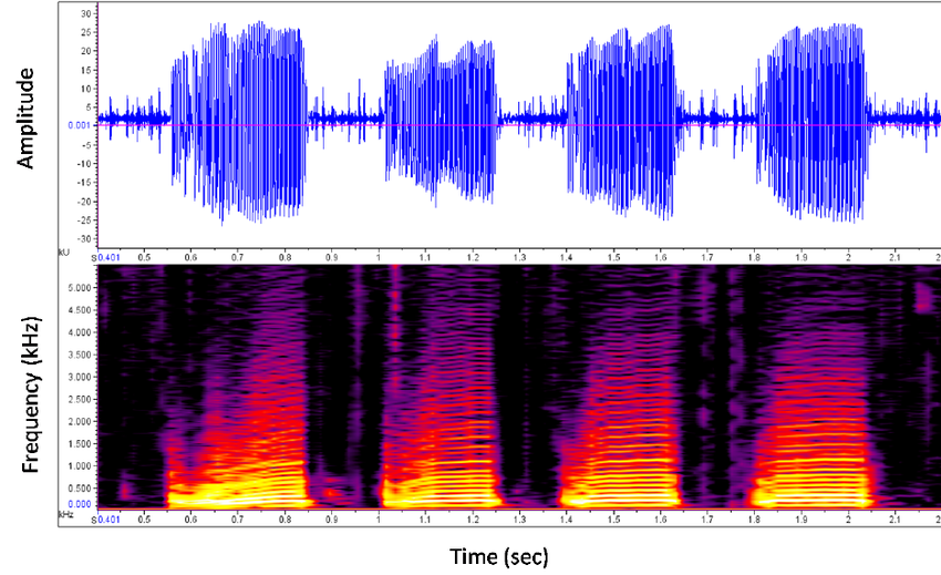
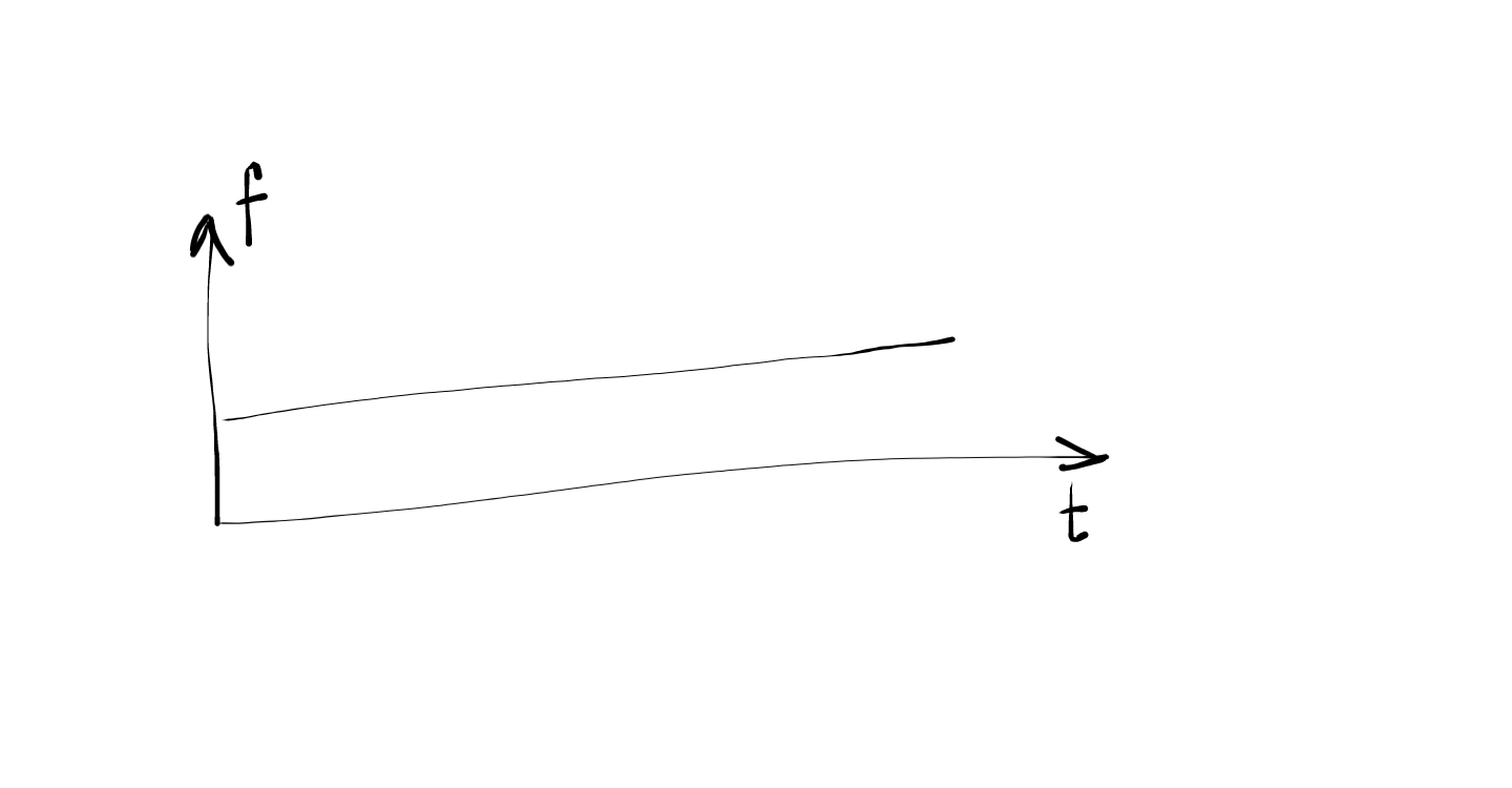
In the previous step, we have amplitude on \(y\) axis and time on \(x\) axis. Now we need to convert it into the frequency scale (called spectrogram). For this, we first take a small piece of time segment (called frame) from the previous step and convert it into a frequency representation. Here, on \(x\) axis we get the series of frames that we’ve sampled. On \(y\) axis, we get the distribution over all frequencies (Like a softmax at each frame step).
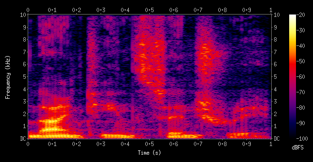
For eg, let us say that the frame we sampled has a \(sine\) curve and that this \(sine\) function has a frequency \(f\) (which is fixed). Therefore, for this frame there will be a single peak at the frequency \(f\) and 0 everywhere else. If the entire waveform is the same \(sine\) graph (i.e every frame in the waveform has the same curve), in each frequency distribution, there will be the same single peak at \(f\). This will result in a horizontal line (just like a softmax).
In this frequency distribution, the max frequency it can take is a specification. Phones usually do \(8kHz\). ASRs like Kaldi and CMUSphinx need recordings at or above \(16kHz\). Normally we record in \(44kHz\) for music.
Sample Numbers:
While converting the audio signal from amplitude domain to the frequency domain, we spoke about taking small time segments called frames (called sampling-rate). If the audio that we have is a \(16kHz\) audio, we have \(16 \times 10^{3}\) numbers for each \(1 s\). Usually, the window size for sampling is \(25 ms\) with a \(10 ms\) step. Hence, each frame size will be \(16 \times 10^{3} \times 25 \times 10^{-3} = 400\). Hence, we will get a vector of size \(400\) every \(10 ms\).
Overview of audio processing
- Dithering: Adding a very small amount of noise to the signal to prevent mathematical issues during feature computation (in particular, taking the logarithm of 0).
- DC-Removal: Removing any constant offset from the waveform.
- Pre-emphasis Filter: Applying a high pass filter to the signal prior to feature extraction to counteract that fact that typically the voiced speech at the lower frequencies has much high energy than the unvoiced speech at high frequencies.
- Mel Filtering: Binning and applying the filter on each frame.
- Log of Mel Frequencies: Taking log of the values from previous step.
At the end of these steps, we get vectors called as MFCC (Mel-frequency cepstral coefficients) vectors which are then used as the representation of the audio. We can think of these MFCC vectors as analogous to word embeddings in the NLP domain.
Cepstral Mean and Variance Normalization (CMVN)
As soon as we dive into any ASR system, we will be accosted with the term CMVN in the pre-processing step right after MFCC generation. It is important to understand the significance of this normalization step and to do that, we need to understand what it is.
Whenever a signal (audio in our case) passes through a noisy channel, the channel introduces some noise to the signal. This is referred to as channel impulse response in signal processing lingo. Whenever an impulse signal is sent through a channel, the channel distorts this impulse in a certain way.
When we record any audio with voice, it consists of the pure voice signal \(x[n]\) and the channel impulse response \(h[n]\). Therefore, the recorded signal is a linear convolution of both of them and is given by,
\[y[n] = x[n] \bigstar h[n]\]
When we take the Fourier Transform of the above signal (which we do to get MFCC), linear convolution becomes simple product.
\[Y[f] = X[f].H[f]\]
Further, in the process of calculating MFCC, we take the logarithm of this value and we end up with,
\[Y[q] = log(Y[f]) = log(X[f].H[f]) = X[q]+H[q]\]
since \(log(a.b) = log(a)+log(b)\).
We can see that any linear convolution distortion in the audio is represented as an addition in the cepstral domain. Let us assume that the channel impulse response is constant for a given channel (This is a strong assumption since we are assuming that the noise component of the channel is going to remain stationary). Then, for a series of audio signals,
\[Y_{i}[q] = X_{i}[q] + H[q]\]
By taking average of all the frames,
\[\frac{1}{N}\sum_{i}Y_{i}[q] = H[q]+\frac{1}{N}\sum_{i}X_{i}[q]\]
If we subtract this mean from each cepstral coefficient, we get,
\[R_{i}[q]=Y_{i}[q]-\frac{1}{N}\sum_{j}Y_{j}[q]\]
\[R_{i}[q]=X_{i}[q] + H[q] - \left ( H[q]+\frac{1}{N}\sum_{j}X_{j}[q] \right )\]
\[R_{i}[q]=X_{i}[q] - \frac{1}{N}\sum_{j}X_{j}[q]\]
In the above equation, we can see that the channel effects (distortions) are removed. In simpler words, subtracting the mean from all cepstral coefficients (such that the mean of all vectors is zero) (this process is called CMVN) removes the channel distortions from the signal and hence is an important pre-processing step in speech recognition.
04 Dec 2018
Automatic Speech Recognition (ASR) systems are used for transcribing spoken text into words/sentences. ASR systems are complex systems consisting of multiple components,
working in tandem to transcribe. In this blog series, I will be exploring the different components of a generic ASR system (although I will be using Kaldi for some
references).
Any ASR system consists of the following basic components:
ASR Resources
Abbreviations
- LVCSR - Large Vocabulary Continuous Speech Recognition
- HMM - Hidden Markov Models
- AM - Acoustic Model
- LM - Language Model
Data Requirements
The following are the data requirements for any ASR system
- Labeled Corpus: Collection of speech audio files and their transcriptions
- Lexicon: Mapping from the word to the series of phones to describe how the word is pronounced.
Not necessary for phonetically written languages like Kannada.
- Data for training Language Model: Large text corpus (to train a statistical language model) in case we are looking to train an ASR system to handle generic/natural language inputs.
If we are looking at constrained ASR systems that are only capable of transcribing a certain set of grammar rules (like PAN numbers, telephone numbers etc),
we can directly write the grammar rules without training a statistical LM and hence this requirement is flexible.
Bayes Rule in ASR
Any ASR follows the following principle.
\[P(S|audio) = \frac{P(audio|S)P(S)}{P(audio)}\]
Here, \(P(S)\) is the LM and \(S\) is the sentence.
\(P(audio)\) is irrelevant since we are taking argmax.
\(P(audio|S)\) is the Acoustic Model. This describes distribution over the acoustic observations \(audio\) given the word sequence \(S\).
This equation is called as the Fundamental Equation of Speech Recognition
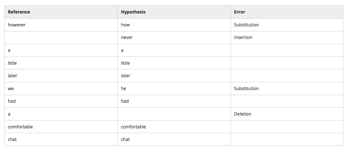
Evaluation
Word Error Rate - \(WER = \frac{N_{sub} + N_{del} + N_{ins}}{N_{\text{reference_sentence}}}\)
Significance Testing
Statistical significance testing involves measuring to what degree the difference between two experiments (or algorithms) can be attributed to actual differences in the two algorithms or are merely the result inherent variability in the data, experimental setup or other factors.
Matched Pairs Testing
07 Oct 2018
This blog is a summary of the ideas outlined in Chomsky’s Syntactic Structures.
Table of Contents
- Language
- Grammar
- Phonemes and Morphemes
- Markov Processes for language generation
- Limitations of Phrase structure description
- Grammatical Transformation
- Procedure for formalizing computational linguistics
- Explanation power of linguistics
- Syntax and Semantics
Language
Any language L is considered to be a set of sentences. Each sentence is finite in length and is constructed out of a finite set of elements (words). A sentence can be a sequence of phonemes or letters in an alphabet.
Grammar
Grammar has no relation to semantic meaning of a sentence. A sentence can be grammatically correct and not have any meaning. Since the probability of grammatically correct and incorrect sentences occurring in a corpus of text is highly dependent on the corpus, we cannot leverage statistics to find out if a sentence is grammatically correct or not. (Although we know that this is not true anymore as we can build robust language models that care capable of probabilistically generating grammatically correct sentences).
Conclusion: Grammar is autonomous and independent of meaning, and that probabilistic models give no particular insight into some of the basic problems of syntactic structure.
Phonemes and Morphemes
Phonemes are smallest elements in pronunciation. Morphemes are smallest elements in words.
Markov Processes for language generation
Chomsky talks of a finite state machine (finite state grammar) that can be used for generation of sentences. He argues that since since English is a non-finite state language, we cannot use a finite state machine to generate English sentences.
-
Finite state language
a[3]b[4] is finite.
-
Infinite state language
a*b* is infinite.
Similarly, the following demonstrates how English is also infinite.
Suppose \(S_{1}\), \(S_{2}\) and \(S_{3}\) are declarative sentences, we can construct the following sentences using grammar rules.
If \(S_{1}\), then \(S_{2}\).
Either \(S_{3}\) or \(S_{4}\).
Each of the above sentence is also declarative and hence can be expanded infinitely.
Limitations of Phrase structure description
-
If there are two sentences of the form Z + X + W and Z + Y + W, we can use the conjunction and and construct a new sentence of the form Z-X+ and +Y-W (Only if X and Y are constituents)
For eg,
the scene - of the movie - was in Chicago
the scene - of the play - was in Chicago
the scene - of the movie and of the play - was in Chicago
The above assumption does not hold true in the following case where X and Y are not constituents
the - liner sailed down the - river
the - tugboat chugged up the - river
the - liner sailed down the and the tugboat chugged up the - river
The limitation in this case is that unless X and Y are constituents, we cannot apply this grammar rule. But it is not possible to incorporate this rule in any
phrase structure grammar. Why? Because we need to know the actual form of the 2 sentences and if X and Y are constituents (for which we need to know their values).
-
Auxilary Verbs
-
Active passive relation
“John admires sincerity” <-> “sincerity admires John”
“sincerity frightens John” <-> “John frightens sincerity”
These examples demonstrate that even though these sentences are not violating any grammar rules, they are semantically incorrect and hence pose limitations to the assumption that grammar does not depend on semantics. These limitations can be overcome by having extra rules (which cannot be incorporated within the grammar itself) over the grammar.
-
In order to overcome the above limitations, we can assume the grammar to have 3 levels of rules:
-
Phrase Structure
-
Transformational Structure
-
Morphophonemics
Given a sentence, we first go through the phrase structure grammar to build a tree and get to the leaf nodes (terminal words).
We then run through the transformational structural rules (both optional and obligatory rules) to transform the set of terminal nodes.
We then apply the morphophonemics to arrive at the final sentence.
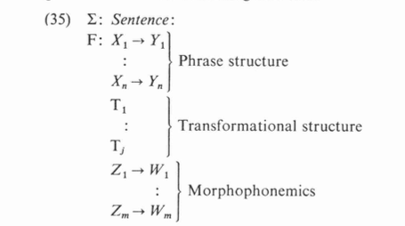
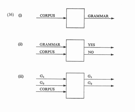
Of the 3 approaches outlined in the diagram above, Chomsky proposes to choose the one in which we can come to a reasonable solution to, hence evaluation. He says, generating (discovery) of the correct grammar given a data corpus is not feasible (we know this is not true now, because we can build language models given a huge corpus).
Explanation power of linguistics
Reason to have a separate representation for morphemes and phonemes is demonstrated here. The phoneme sequence /eneym/ can be understood ambiguously as both “a name” or a “an aim”.
If our grammar is only a single level system dealing with only phonemes, we have no way of representing this ambiguity. Therefore we need a second morphological layer.
Syntax and Semantics
The three levels of parsing of grammar gives us the ability to perform the following representations:
-
Represent sentences that can be understood in more than one way ambiguously.
-
Represent two sentences that are understood in a similar manner similarly on the transformational level.
Chomsky argues that there cannot be any relation between semantics and grammar i.e the burden of proof lies on the linguist claiming that the grammar should be dependent
on semantics.
Assertions supporting dependence of grammar on meaning:
-
Two utterances are phonemically distinct if and only if they differ in meanings
This is refuted because of synonyms (utterance tokens that are phonemically different but means the same thing) and homonyms (utterance tokens that are phonemically
identical but differ in meaning)
-
Morphemes are the smallest elements that have meanings
This is refuted because morpheme such as gl- in “gleam”, “glimmer” and “glow” does not carry any meaning in itself.
-
Grammatical sentences are those that have semantic significance
-
NP - VP -> actor-action
“the fighting stopped” has no actor-action relation
-
Verb - NP -> action-goal or action-object of action
“I missed the train” has no action-goal relation
-
Active sentence and corresponding passive sentence are synonymous
“everyone in the room knows at least two languages” is not synonymous to “at least two languages are known by everyone in the room”
02 Oct 2018
In the previous blog post on Transfer Learning, we discovered how pre-trained models can be leveraged in our applications to save on train time, data, compute and other resources along with the added benefit of better performance. In this blog post, I will be demonstrating how to use ELMo Embeddings in Keras.
Pre-trained ELMo Embeddings are freely available as a Tensorflow Hub Module. I prefer Keras for quick experimentation and iteration and hence I was looking at ways to use these models from the Hub directly in my Keras project. Unfortunately, this is not as straightforward as it initially seems to be. ELMo has 4 trainable parameters that needs to be trained/fine-tuned with your custom dataset. The expected behaviour in this scenario is that these weights get updated as part of the learning procedure of the entire network. On the contrary, these 4 learnable parameters refused to get updated and hence, I decided to write a custom layer in Keras that updates these weights manually.
Here is the code:
elmo_model = hub.Module("https://tfhub.dev/google/elmo/2", trainable=True)
sess = tf.Session()

K.set_session(sess)
# Initialize sessions
sess.run(tf.global_variables_initializer())
sess.run(tf.tables_initializer())

class KerasLayer(Layer):

    def __init__(self, output_dim, **kwargs):
        self.output_dim = output_dim
        super(MyLayer, self).__init__(**kwargs)

    def build(self, input_shape):
        # Create a trainable weight variable for this layer.

        # These are the 3 trainable weights for word_embedding, lstm_output1 and lstm_output2
        self.kernel1 = self.add_weight(name='kernel1',
                                       shape=(3,),
                                      initializer='uniform',
                                      trainable=True)
        # This is the bias weight
        self.kernel2 = self.add_weight(name='kernel2',
                                       shape=(),
                                      initializer='uniform',
                                      trainable=True)
        super(MyLayer, self).build(input_shape)

    def call(self, x):
        # Get all the outputs of elmo_model
        model =  elmo_model(tf.squeeze(tf.cast(x, tf.string)), signature="default", as_dict=True)

        # Embedding activation output
        activation1 = model["word_emb"]

        # First LSTM layer output
        activation2 = model["lstm_outputs1"]

        # Second LSTM layer output
        activation3 = model["lstm_outputs2"]

        activation2 = tf.reduce_mean(activation2, axis=1)
        activation3 = tf.reduce_mean(activation3, axis=1)

        mul1 = tf.scalar_mul(self.kernel1[0], activation1)
        mul2 = tf.scalar_mul(self.kernel1[1], activation2)
        mul3 = tf.scalar_mul(self.kernel1[2], activation3)

        sum_vector = tf.add(mul2, mul3)

        return tf.scalar_mul(self.kernel2, sum_vector)

    def compute_output_shape(self, input_shape):
        return (input_shape[0], self.output_dim)

input_text = layers.Input(shape=(1,), dtype=tf.string)
custom_layer = KerasLayer(output_dim=1024, trainable=True)(input_text)
pred = layers.Dense(1, activation='sigmoid', trainable=False)(custom_layer)

model = Model(inputs=input_text, outputs=pred)

model.compile(loss='binary_crossentropy', optimizer='adam', metrics=['accuracy'])
print(model.summary())
model.fit(inp, target, epochs=15, batch_size=32)